15 Insights from Rhode Island School Enrollment Data
Source:vignettes/enrollment_hooks.Rmd
enrollment_hooks.Rmd
library(rischooldata)
library(dplyr)
library(tidyr)
library(ggplot2)

theme_set(theme_minimal(base_size = 14))
This vignette explores Rhode Island’s public school enrollment data, surfacing key trends and demographic patterns across 14 years of data (2012-2025). State-level demographics are available from 2012 onward.
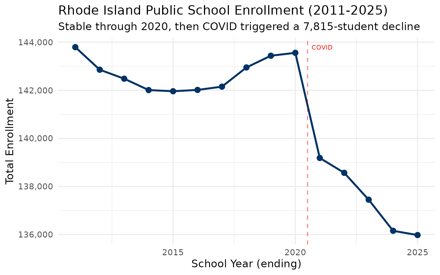
1. Rhode Island lost 7,815 students since 2011
Rhode Island’s public school enrollment hovered near 143,000 students from 2011 through 2020, then COVID triggered a sharp drop that the state has not recovered from.
enr <- fetch_enr_multi(2012:2025, use_cache = TRUE)
enr_2011 <- fetch_enr(2011, use_cache = TRUE)

state_totals <- bind_rows(
  enr_2011 |>
    filter(is_state, subgroup == "total_enrollment", grade_level == "TOTAL") |>
    select(end_year, n_students),
  enr |>
    filter(is_state, subgroup == "total_enrollment", grade_level == "TOTAL") |>
    select(end_year, n_students)
) |>
  arrange(end_year) |>
  mutate(change = n_students - lag(n_students),
         pct_change = round(change / lag(n_students) * 100, 2))

stopifnot(nrow(state_totals) > 0)
state_totals
#>    end_year n_students change pct_change
#> 1      2011     143793     NA         NA
#> 2      2012     142854   -939      -0.65
#> 3      2013     142481   -373      -0.26
#> 4      2014     142008   -473      -0.33
#> 5      2015     141959    -49      -0.03
#> 6      2016     142014     55       0.04
#> 7      2017     142150    136       0.10
#> 8      2018     142949    799       0.56
#> 9      2019     143436    487       0.34
#> 10     2020     143557    121       0.08
#> 11     2021     139184  -4373      -3.05
#> 12     2022     138566   -618      -0.44
#> 13     2023     137449  -1117      -0.81
#> 14     2024     136154  -1295      -0.94
#> 15     2025     135978   -176      -0.13
print(state_totals)
#>    end_year n_students change pct_change
#> 1      2011     143793     NA         NA
#> 2      2012     142854   -939      -0.65
#> 3      2013     142481   -373      -0.26
#> 4      2014     142008   -473      -0.33
#> 5      2015     141959    -49      -0.03
#> 6      2016     142014     55       0.04
#> 7      2017     142150    136       0.10
#> 8      2018     142949    799       0.56
#> 9      2019     143436    487       0.34
#> 10     2020     143557    121       0.08
#> 11     2021     139184  -4373      -3.05
#> 12     2022     138566   -618      -0.44
#> 13     2023     137449  -1117      -0.81
#> 14     2024     136154  -1295      -0.94
#> 15     2025     135978   -176      -0.13

ggplot(state_totals, aes(x = end_year, y = n_students)) +
  geom_line(linewidth = 1.2, color = "#003366") +
  geom_point(size = 3, color = "#003366") +
  geom_vline(xintercept = 2020.5, linetype = "dashed", color = "red", alpha = 0.5) +
  annotate("text", x = 2020.5, y = max(state_totals$n_students), label = "COVID", hjust = -0.2, color = "red", size = 3) +
  scale_y_continuous(labels = scales::comma) +
  labs(
    title = "Rhode Island Public School Enrollment (2011-2025)",
    subtitle = "Stable through 2020, then COVID triggered a 7,815-student decline",
    x = "School Year (ending)",
    y = "Total Enrollment"
  )
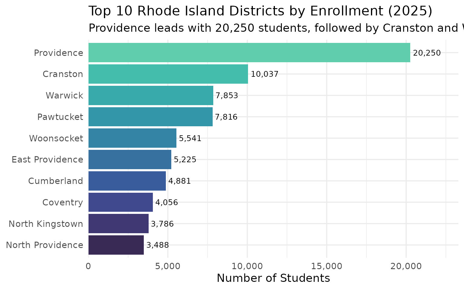
2. Providence dominates, serving 15% of students
Providence is Rhode Island’s largest district by far, enrolling over 20,000 students–about one in seven Rhode Island students.
enr_2025 <- fetch_enr(2025, use_cache = TRUE)

top_districts <- enr_2025 |>
  filter(is_district, subgroup == "total_enrollment", grade_level == "TOTAL") |>
  arrange(desc(n_students)) |>
  head(10) |>
  select(district_name, n_students)

stopifnot(nrow(top_districts) > 0)
top_districts
#>       district_name n_students
#> 1        Providence      20250
#> 2          Cranston      10037
#> 3           Warwick       7853
#> 4         Pawtucket       7816
#> 5        Woonsocket       5541
#> 6   East Providence       5225
#> 7        Cumberland       4881
#> 8          Coventry       4056
#> 9   North Kingstown       3786
#> 10 North Providence       3488
print(top_districts)
#>       district_name n_students
#> 1        Providence      20250
#> 2          Cranston      10037
#> 3           Warwick       7853
#> 4         Pawtucket       7816
#> 5        Woonsocket       5541
#> 6   East Providence       5225
#> 7        Cumberland       4881
#> 8          Coventry       4056
#> 9   North Kingstown       3786
#> 10 North Providence       3488

top_districts |>
  mutate(district_name = forcats::fct_reorder(district_name, n_students)) |>
  ggplot(aes(x = n_students, y = district_name, fill = district_name)) +
  geom_col(show.legend = FALSE) +
  geom_text(aes(label = scales::comma(n_students)), hjust = -0.1, size = 3.5) +
  scale_x_continuous(labels = scales::comma, expand = expansion(mult = c(0, 0.15))) +
  scale_fill_viridis_d(option = "mako", begin = 0.2, end = 0.8) +
  labs(
    title = "Top 10 Rhode Island Districts by Enrollment (2025)",
    subtitle = "Providence leads with 20,250 students, followed by Cranston and Warwick",
    x = "Number of Students",
    y = NULL
  )
3. Providence lost 3,705 students since 2019
Providence lost nearly 4,000 students between 2019 and 2025, a 15% decline driven by pandemic disruption and demographic shifts.
covid_enr <- fetch_enr_multi(2019:2025, use_cache = TRUE)

providence_trend <- covid_enr |>
  filter(district_name == "Providence", is_district,
         subgroup == "total_enrollment", grade_level == "TOTAL") |>
  select(end_year, n_students) |>
  mutate(change = n_students - first(n_students))

stopifnot(nrow(providence_trend) > 0)
providence_trend
#>   end_year n_students change
#> 1     2019      23955      0
#> 2     2020      23836   -119
#> 3     2021      22440  -1515
#> 4     2022      21656  -2299
#> 5     2023      20725  -3230
#> 6     2024      19856  -4099
#> 7     2025      20250  -3705
4. Hispanic students now 31% of enrollment
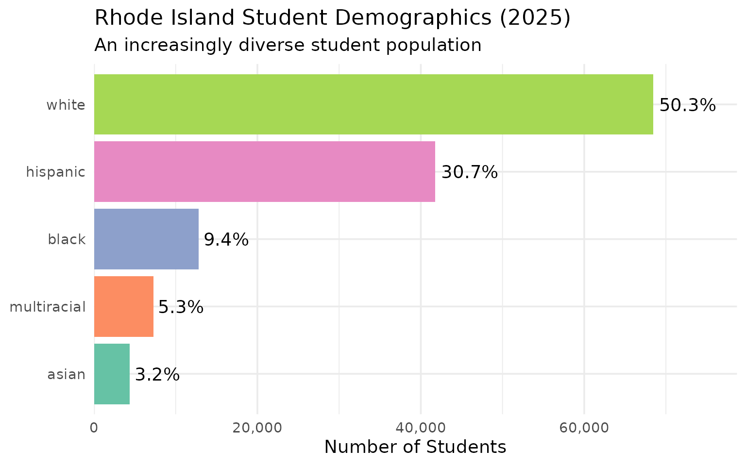
Rhode Island’s Hispanic population has grown dramatically, from 22% in 2012 to nearly 31% today, making it one of the fastest-growing demographic groups in the state.
demographics <- enr_2025 |>
  filter(is_state, grade_level == "TOTAL",
         subgroup %in% c("white", "black", "hispanic", "asian", "multiracial")) |>
  mutate(pct = round(pct * 100, 1)) |>
  select(subgroup, n_students, pct) |>
  arrange(desc(n_students))

stopifnot(nrow(demographics) > 0)
demographics
#>      subgroup n_students  pct
#> 1       white      68431 50.3
#> 2    hispanic      41785 30.7
#> 3       black      12818  9.4
#> 4 multiracial       7273  5.3
#> 5       asian       4391  3.2
print(demographics)
#>      subgroup n_students  pct
#> 1       white      68431 50.3
#> 2    hispanic      41785 30.7
#> 3       black      12818  9.4
#> 4 multiracial       7273  5.3
#> 5       asian       4391  3.2

demographics |>
  mutate(subgroup = forcats::fct_reorder(subgroup, n_students)) |>
  ggplot(aes(x = n_students, y = subgroup, fill = subgroup)) +
  geom_col(show.legend = FALSE) +
  geom_text(aes(label = paste0(pct, "%")), hjust = -0.1) +
  scale_x_continuous(labels = scales::comma, expand = expansion(mult = c(0, 0.15))) +
  scale_fill_brewer(palette = "Set2") +
  labs(
    title = "Rhode Island Student Demographics (2025)",
    subtitle = "An increasingly diverse student population",
    x = "Number of Students",
    y = NULL
  )
5. Central Falls enrollment held steady despite statewide decline
While Rhode Island lost students statewide, tiny Central Falls – one of the nation’s poorest cities – maintained enrollment near 2,600 students, reflecting its role as a gateway community for immigrant families.
cf_trend <- fetch_enr_multi(2015:2025, use_cache = TRUE) |>
filter(grepl("Central Falls", district_name), is_district,
subgroup == "total_enrollment", grade_level == "TOTAL") |>
select(end_year, n_students) |>
mutate(change = n_students - first(n_students))
stopifnot(nrow(cf_trend) > 0)
cf_trend
#> end_year n_students change
#> 1 2015 2683 0
#> 2 2016 2657 -26
#> 3 2017 2589 -94
#> 4 2018 2518 -165
#> 5 2019 2695 12
#> 6 2020 2878 195
#> 7 2021 2780 97
#> 8 2022 2701 18
#> 9 2023 2596 -87
#> 10 2024 2539 -144
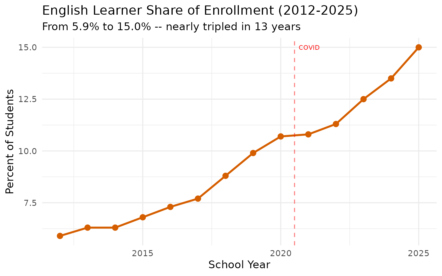
#> 11 2025 2560 -1236. English learners tripled statewide since 2012
Rhode Island’s English learner population surged from 5.9% to 15.0% of enrollment between 2012 and 2025 – a statewide transformation driven by immigration.
lep_trend <- enr |>
  filter(is_state, grade_level == "TOTAL", subgroup == "lep") |>
  select(end_year, n_students, pct) |>
  mutate(pct = round(pct * 100, 1))

stopifnot(nrow(lep_trend) > 0)
lep_trend
#>    end_year n_students  pct
#> 1      2012       8436  5.9
#> 2      2013       8913  6.3
#> 3      2014       8980  6.3
#> 4      2015       9643  6.8
#> 5      2016      10341  7.3
#> 6      2017      10888  7.7
#> 7      2018      12629  8.8
#> 8      2019      14138  9.9
#> 9      2020      15377 10.7
#> 10     2021      15084 10.8
#> 11     2022      15721 11.3
#> 12     2023      17226 12.5
#> 13     2024      18422 13.5
#> 14     2025      20352 15.0
print(lep_trend)
#>    end_year n_students  pct
#> 1      2012       8436  5.9
#> 2      2013       8913  6.3
#> 3      2014       8980  6.3
#> 4      2015       9643  6.8
#> 5      2016      10341  7.3
#> 6      2017      10888  7.7
#> 7      2018      12629  8.8
#> 8      2019      14138  9.9
#> 9      2020      15377 10.7
#> 10     2021      15084 10.8
#> 11     2022      15721 11.3
#> 12     2023      17226 12.5
#> 13     2024      18422 13.5
#> 14     2025      20352 15.0

lep_trend |>
  ggplot(aes(x = end_year, y = pct)) +
  geom_line(linewidth = 1.2, color = "#D55E00") +
  geom_point(size = 3, color = "#D55E00") +
  geom_vline(xintercept = 2020.5, linetype = "dashed", color = "red", alpha = 0.5) +
  annotate("text", x = 2020.5, y = max(lep_trend$pct), label = "COVID", hjust = -0.2, color = "red", size = 3) +
  labs(
    title = "English Learner Share of Enrollment (2012-2025)",
    subtitle = "From 5.9% to 15.0% -- nearly tripled in 13 years",
    x = "School Year",
    y = "Percent of Students"
  )
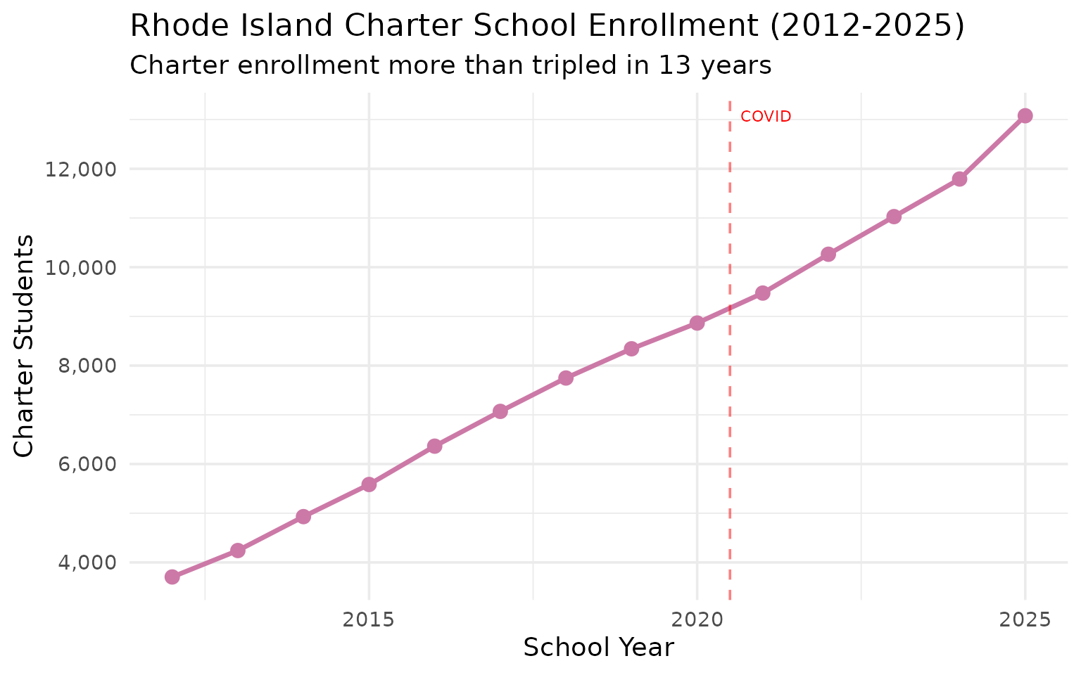
7. Charter schools serve 13,000+ students across 25 schools
Rhode Island’s charter sector has grown from 3,705 students in 2012 to 13,078 in 2025, now serving 9.6% of all public school students.
charters <- enr_2025 |>
  filter(is_charter, is_district, subgroup == "total_enrollment", grade_level == "TOTAL") |>
  summarize(
    n_charters = n(),
    total_students = sum(n_students, na.rm = TRUE)
  )

stopifnot(nrow(charters) > 0)
charters
#>   n_charters total_students
#> 1         25          13078
charter_trend <- enr |>
  filter(is_charter, is_district, subgroup == "total_enrollment", grade_level == "TOTAL") |>
  group_by(end_year) |>
  summarize(
    n_charters = n(),
    total_students = sum(n_students, na.rm = TRUE),
    .groups = "drop"
  )

stopifnot(nrow(charter_trend) > 0)
print(charter_trend)
#> # A tibble: 14 × 3
#>    end_year n_charters total_students
#>       <int>      <int>          <dbl>
#>  1     2012         14           3705
#>  2     2013         14           4242
#>  3     2014         16           4931
#>  4     2015         19           5584
#>  5     2016         19           6363
#>  6     2017         19           7070
#>  7     2018         19           7748
#>  8     2019         20           8342
#>  9     2020         20           8865
#> 10     2021         20           9474
#> 11     2022         22          10263
#> 12     2023         24          11028
#> 13     2024         24          11792
#> 14     2025         25          13078

charter_trend |>
  ggplot(aes(x = end_year, y = total_students)) +
  geom_line(linewidth = 1.2, color = "#CC79A7") +
  geom_point(size = 3, color = "#CC79A7") +
  geom_vline(xintercept = 2020.5, linetype = "dashed", color = "red", alpha = 0.5) +
  annotate("text", x = 2020.5, y = max(charter_trend$total_students), label = "COVID", hjust = -0.2, color = "red", size = 3) +
  scale_y_continuous(labels = scales::comma) +
  labs(
    title = "Rhode Island Charter School Enrollment (2012-2025)",
    subtitle = "Charter enrollment more than tripled in 13 years",
    x = "School Year",
    y = "Charter Students"
  )
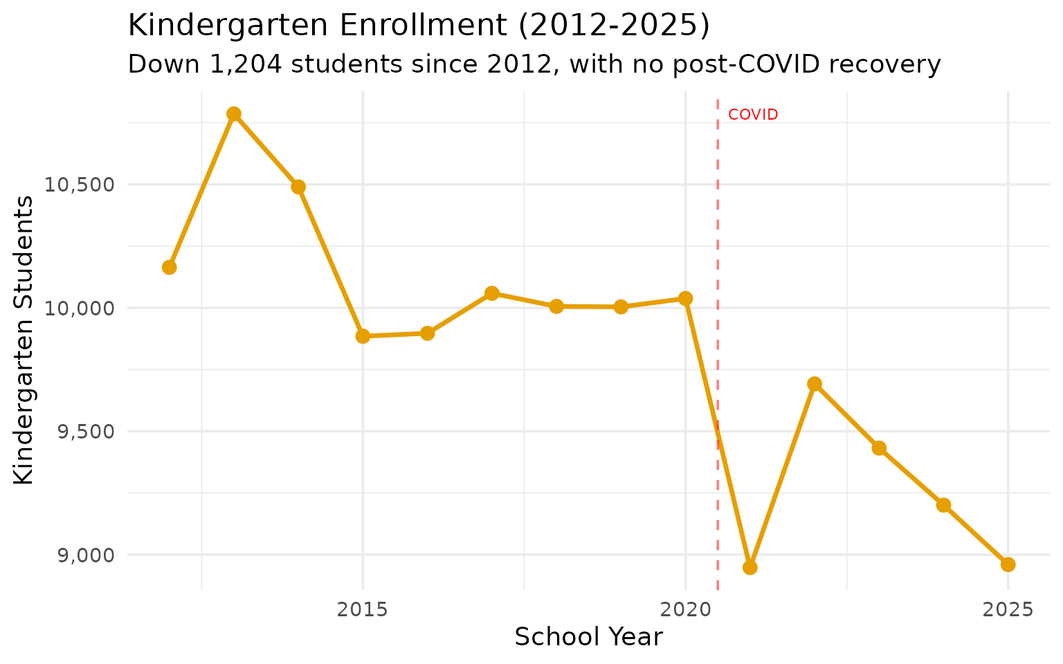
8. Kindergarten enrollment down 12% since 2012
After sharp COVID-era drops, kindergarten enrollment has continued to decline rather than recovering, suggesting a longer-term demographic shift beyond pandemic effects.
k_trend <- enr |>
  filter(is_state, subgroup == "total_enrollment", grade_level == "K") |>
  select(end_year, n_students) |>
  mutate(change = n_students - first(n_students))

stopifnot(nrow(k_trend) > 0)
k_trend
#>    end_year n_students change
#> 1      2012      10164      0
#> 2      2013      10786    622
#> 3      2014      10490    326
#> 4      2015       9885   -279
#> 5      2016       9897   -267
#> 6      2017      10059   -105
#> 7      2018      10006   -158
#> 8      2019      10004   -160
#> 9      2020      10038   -126
#> 10     2021       8948  -1216
#> 11     2022       9692   -472
#> 12     2023       9432   -732
#> 13     2024       9201   -963
#> 14     2025       8960  -1204
print(k_trend)
#>    end_year n_students change
#> 1      2012      10164      0
#> 2      2013      10786    622
#> 3      2014      10490    326
#> 4      2015       9885   -279
#> 5      2016       9897   -267
#> 6      2017      10059   -105
#> 7      2018      10006   -158
#> 8      2019      10004   -160
#> 9      2020      10038   -126
#> 10     2021       8948  -1216
#> 11     2022       9692   -472
#> 12     2023       9432   -732
#> 13     2024       9201   -963
#> 14     2025       8960  -1204

k_trend |>
  ggplot(aes(x = end_year, y = n_students)) +
  geom_line(linewidth = 1.2, color = "#E69F00") +
  geom_point(size = 3, color = "#E69F00") +
  geom_vline(xintercept = 2020.5, linetype = "dashed", color = "red", alpha = 0.5) +
  annotate("text", x = 2020.5, y = max(k_trend$n_students), label = "COVID", hjust = -0.2, color = "red", size = 3) +
  scale_y_continuous(labels = scales::comma) +
  labs(
    title = "Kindergarten Enrollment (2012-2025)",
    subtitle = "Down 1,204 students since 2012, with no post-COVID recovery",
    x = "School Year",
    y = "Kindergarten Students"
  )
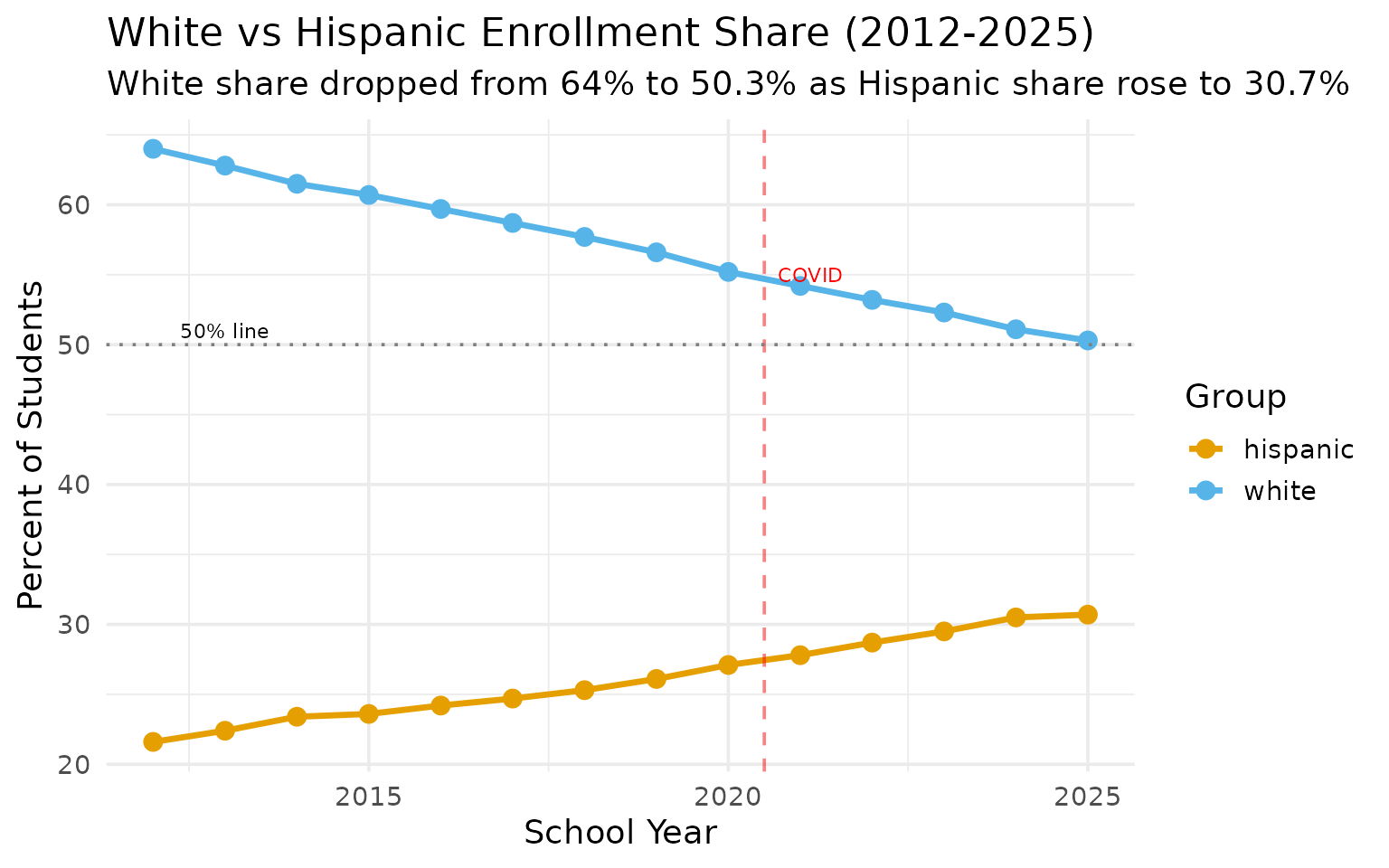
9. White students narrowly hold majority at 50.3%
Rhode Island is on the cusp of a demographic milestone – white students still hold a slim majority at 50.3%, but Hispanic enrollment has grown from 21.6% to 30.7% since 2012.
race_trends <- enr |>
  filter(is_state, grade_level == "TOTAL",
         subgroup %in% c("white", "hispanic")) |>
  select(end_year, subgroup, pct) |>
  mutate(pct = round(pct * 100, 1)) |>
  pivot_wider(names_from = subgroup, values_from = pct)

stopifnot(nrow(race_trends) > 0)
race_trends
#> # A tibble: 14 × 3
#>    end_year white hispanic
#>       <int> <dbl>    <dbl>
#>  1     2012  64       21.6
#>  2     2013  62.8     22.4
#>  3     2014  61.5     23.4
#>  4     2015  60.7     23.6
#>  5     2016  59.7     24.2
#>  6     2017  58.7     24.7
#>  7     2018  57.7     25.3
#>  8     2019  56.6     26.1
#>  9     2020  55.2     27.1
#> 10     2021  54.2     27.8
#> 11     2022  53.2     28.7
#> 12     2023  52.3     29.5
#> 13     2024  51.1     30.5
#> 14     2025  50.3     30.7
print(race_trends)
#> # A tibble: 14 × 3
#>    end_year white hispanic
#>       <int> <dbl>    <dbl>
#>  1     2012  64       21.6
#>  2     2013  62.8     22.4
#>  3     2014  61.5     23.4
#>  4     2015  60.7     23.6
#>  5     2016  59.7     24.2
#>  6     2017  58.7     24.7
#>  7     2018  57.7     25.3
#>  8     2019  56.6     26.1
#>  9     2020  55.2     27.1
#> 10     2021  54.2     27.8
#> 11     2022  53.2     28.7
#> 12     2023  52.3     29.5
#> 13     2024  51.1     30.5
#> 14     2025  50.3     30.7

race_long <- enr |>
  filter(is_state, grade_level == "TOTAL",
         subgroup %in% c("white", "hispanic")) |>
  select(end_year, subgroup, pct) |>
  mutate(pct = round(pct * 100, 1))

race_long |>
  ggplot(aes(x = end_year, y = pct, color = subgroup)) +
  geom_line(linewidth = 1.2) +
  geom_point(size = 3) +
  geom_vline(xintercept = 2020.5, linetype = "dashed", color = "red", alpha = 0.5) +
  annotate("text", x = 2020.5, y = 55, label = "COVID", hjust = -0.2, color = "red", size = 3) +
  geom_hline(yintercept = 50, linetype = "dotted", color = "gray50") +
  annotate("text", x = 2013, y = 51, label = "50% line", size = 3) +
  scale_color_manual(values = c("white" = "#56B4E9", "hispanic" = "#E69F00")) +
  labs(
    title = "White vs Hispanic Enrollment Share (2012-2025)",
    subtitle = "White share dropped from 64% to 50.3% as Hispanic share rose to 30.7%",
    x = "School Year",
    y = "Percent of Students",
    color = "Group"
  )
10. 64 districts in America’s smallest state
Rhode Island reports 64 districts (including charter schools), with sizes ranging from Providence’s 20,250 students to New Shoreham’s 126.
size_buckets <- enr_2025 |>
filter(is_district, subgroup == "total_enrollment", grade_level == "TOTAL") |>
mutate(size_bucket = case_when(
n_students < 1000 ~ "Small (<1K)",
n_students < 5000 ~ "Medium (1K-5K)",
n_students < 10000 ~ "Large (5K-10K)",
TRUE ~ "Very Large (10K+)"
)) |>
count(size_bucket) |>
mutate(size_bucket = factor(size_bucket, levels = c("Small (<1K)", "Medium (1K-5K)", "Large (5K-10K)", "Very Large (10K+)")))
stopifnot(nrow(size_buckets) > 0)
size_buckets
#> size_bucket n
#> 1 Large (5K-10K) 4
#> 2 Medium (1K-5K) 26
#> 3 Small (<1K) 32
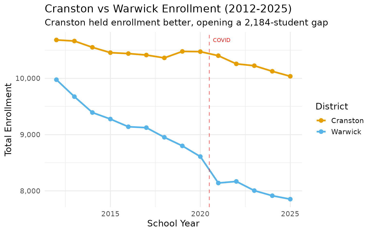
#> 4 Very Large (10K+) 211. Cranston pulls away from Warwick
Cranston and Warwick were Rhode Island’s largest suburban districts at similar sizes in 2011, but Cranston has held enrollment better, opening a 2,184-student gap by 2025.
warwick_cranston <- fetch_enr_multi(2012:2025, use_cache = TRUE) |>
  filter(district_name %in% c("Warwick", "Cranston"), is_district,
         subgroup == "total_enrollment", grade_level == "TOTAL") |>
  select(end_year, district_name, n_students)

stopifnot(nrow(warwick_cranston) > 0)
warwick_cranston |>
  tidyr::pivot_wider(names_from = district_name, values_from = n_students)
#> # A tibble: 14 × 3
#>    end_year Cranston Warwick
#>       <int>    <dbl>   <dbl>
#>  1     2012    10683    9977
#>  2     2013    10664    9675
#>  3     2014    10552    9393
#>  4     2015    10457    9277
#>  5     2016    10441    9140
#>  6     2017    10415    9124
#>  7     2018    10364    8953
#>  8     2019    10479    8800
#>  9     2020    10475    8610
#> 10     2021    10403    8140
#> 11     2022    10258    8168
#> 12     2023    10225    8005
#> 13     2024    10126    7914
#> 14     2025    10037    7853
wc_wide <- warwick_cranston |>
  tidyr::pivot_wider(names_from = district_name, values_from = n_students)
print(wc_wide)
#> # A tibble: 14 × 3
#>    end_year Cranston Warwick
#>       <int>    <dbl>   <dbl>
#>  1     2012    10683    9977
#>  2     2013    10664    9675
#>  3     2014    10552    9393
#>  4     2015    10457    9277
#>  5     2016    10441    9140
#>  6     2017    10415    9124
#>  7     2018    10364    8953
#>  8     2019    10479    8800
#>  9     2020    10475    8610
#> 10     2021    10403    8140
#> 11     2022    10258    8168
#> 12     2023    10225    8005
#> 13     2024    10126    7914
#> 14     2025    10037    7853

warwick_cranston |>
  ggplot(aes(x = end_year, y = n_students, color = district_name)) +
  geom_line(linewidth = 1.2) +
  geom_point(size = 2.5) +
  geom_vline(xintercept = 2020.5, linetype = "dashed", color = "red", alpha = 0.5) +
  annotate("text", x = 2020.5, y = max(warwick_cranston$n_students), label = "COVID", hjust = -0.2, color = "red", size = 3) +
  scale_y_continuous(labels = scales::comma) +
  scale_color_manual(values = c("Cranston" = "#E69F00", "Warwick" = "#56B4E9")) +
  labs(
    title = "Cranston vs Warwick Enrollment (2012-2025)",
    subtitle = "Cranston held enrollment better, opening a 2,184-student gap",
    x = "School Year",
    y = "Total Enrollment",
    color = "District"
  )
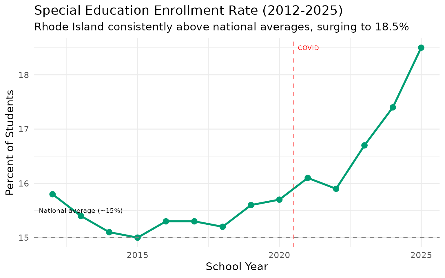
12. Special education rate surged to 18.5%
Rhode Island’s special education identification rate has climbed from 15.8% in 2012 to 18.5% in 2025 – well above the national average of about 15%.
sped_trends <- enr |>
  filter(is_state, grade_level == "TOTAL", subgroup == "special_ed") |>
  select(end_year, n_students, pct) |>
  mutate(pct = round(pct * 100, 1))

stopifnot(nrow(sped_trends) > 0)
sped_trends
#>    end_year n_students  pct
#> 1      2012      22510 15.8
#> 2      2013      21994 15.4
#> 3      2014      21434 15.1
#> 4      2015      21308 15.0
#> 5      2016      21714 15.3
#> 6      2017      21685 15.3
#> 7      2018      21659 15.2
#> 8      2019      22417 15.6
#> 9      2020      22517 15.7
#> 10     2021      22427 16.1
#> 11     2022      22083 15.9
#> 12     2023      22950 16.7
#> 13     2024      23711 17.4
#> 14     2025      25140 18.5
print(sped_trends)
#>    end_year n_students  pct
#> 1      2012      22510 15.8
#> 2      2013      21994 15.4
#> 3      2014      21434 15.1
#> 4      2015      21308 15.0
#> 5      2016      21714 15.3
#> 6      2017      21685 15.3
#> 7      2018      21659 15.2
#> 8      2019      22417 15.6
#> 9      2020      22517 15.7
#> 10     2021      22427 16.1
#> 11     2022      22083 15.9
#> 12     2023      22950 16.7
#> 13     2024      23711 17.4
#> 14     2025      25140 18.5

sped_trends |>
  ggplot(aes(x = end_year, y = pct)) +
  geom_line(linewidth = 1.2, color = "#009E73") +
  geom_point(size = 3, color = "#009E73") +
  geom_vline(xintercept = 2020.5, linetype = "dashed", color = "red", alpha = 0.5) +
  annotate("text", x = 2020.5, y = max(sped_trends$pct), label = "COVID", hjust = -0.2, color = "red", size = 3) +
  geom_hline(yintercept = 15, linetype = "dashed", color = "gray50") +
  annotate("text", x = 2013, y = 15.5, label = "National average (~15%)", size = 3) +
  labs(
    title = "Special Education Enrollment Rate (2012-2025)",
    subtitle = "Rhode Island consistently above national averages, surging to 18.5%",
    x = "School Year",
    y = "Percent of Students"
  )
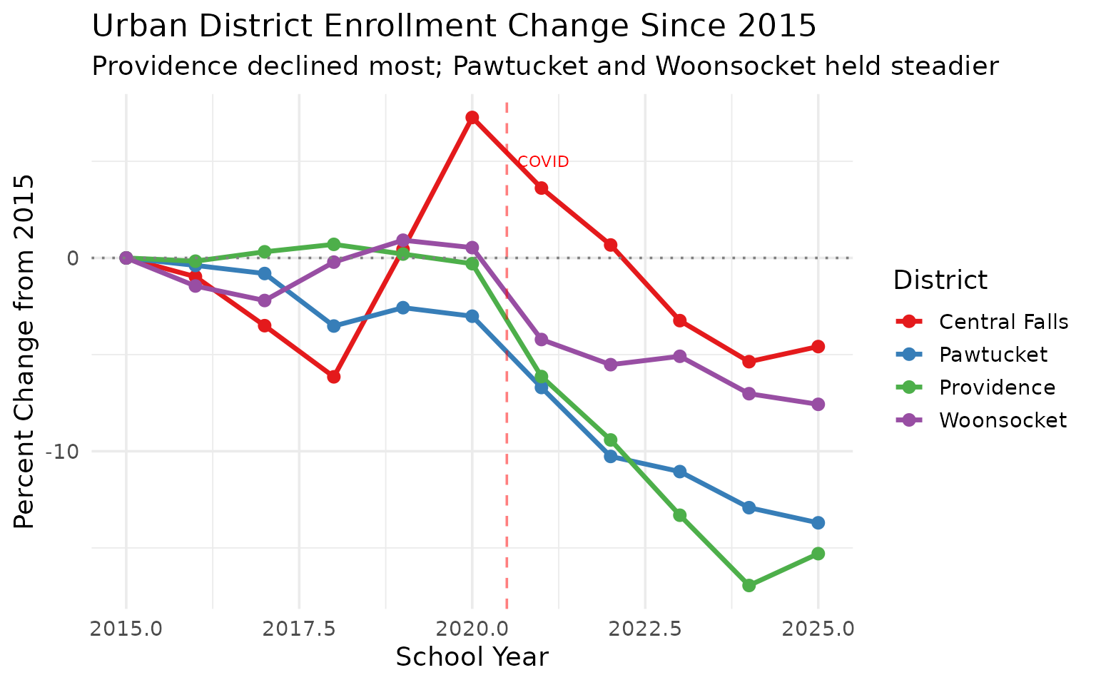
13. Pawtucket holds its ground as the 4th-largest district
Pawtucket often gets overlooked between Providence and Central Falls, but with 7,816 students it is Rhode Island’s 4th-largest district and a key urban center.
pawtucket_trend <- fetch_enr_multi(2015:2025, use_cache = TRUE) |>
  filter(grepl("Pawtucket", district_name), is_district,
         subgroup == "total_enrollment", grade_level == "TOTAL") |>
  select(end_year, n_students) |>
  mutate(change = n_students - first(n_students))

stopifnot(nrow(pawtucket_trend) > 0)
pawtucket_trend
#>    end_year n_students change
#> 1      2015       9057      0
#> 2      2016       9022    -35
#> 3      2017       8984    -73
#> 4      2018       8738   -319
#> 5      2019       8824   -233
#> 6      2020       8784   -273
#> 7      2021       8450   -607
#> 8      2022       8127   -930
#> 9      2023       8056  -1001
#> 10     2024       7887  -1170
#> 11     2025       7816  -1241
print(pawtucket_trend)
#>    end_year n_students change
#> 1      2015       9057      0
#> 2      2016       9022    -35
#> 3      2017       8984    -73
#> 4      2018       8738   -319
#> 5      2019       8824   -233
#> 6      2020       8784   -273
#> 7      2021       8450   -607
#> 8      2022       8127   -930
#> 9      2023       8056  -1001
#> 10     2024       7887  -1170
#> 11     2025       7816  -1241

# Compare urban district enrollment trends
urban_trends <- fetch_enr_multi(2015:2025, use_cache = TRUE) |>
  filter(district_name %in% c("Providence", "Pawtucket", "Central Falls", "Woonsocket"),
         is_district, grade_level == "TOTAL", subgroup == "total_enrollment") |>
  select(end_year, district_name, n_students) |>
  group_by(district_name) |>
  mutate(pct_change = (n_students / first(n_students) - 1) * 100)

stopifnot(nrow(urban_trends) > 0)

urban_trends |>
  ggplot(aes(x = end_year, y = pct_change, color = district_name)) +
  geom_line(linewidth = 1.2) +
  geom_point(size = 2.5) +
  geom_vline(xintercept = 2020.5, linetype = "dashed", color = "red", alpha = 0.5) +
  annotate("text", x = 2020.5, y = 5, label = "COVID", hjust = -0.2, color = "red", size = 3) +
  geom_hline(yintercept = 0, linetype = "dotted", color = "gray50") +
  scale_color_brewer(palette = "Set1") +
  labs(
    title = "Urban District Enrollment Change Since 2015",
    subtitle = "Providence declined most; Pawtucket and Woonsocket held steadier",
    x = "School Year",
    y = "Percent Change from 2015",
    color = "District"
  )
14. Newport lost 277 students since 2015
Newport’s famous tourism economy masks significant educational challenges – the district has lost 13% of its enrollment since 2015.
newport_trend <- fetch_enr_multi(2015:2025, use_cache = TRUE) |>
  filter(grepl("Newport", district_name), is_district,
         subgroup == "total_enrollment", grade_level == "TOTAL") |>
  select(end_year, n_students) |>
  mutate(change = n_students - first(n_students))

stopifnot(nrow(newport_trend) > 0)
newport_trend
#>    end_year n_students change
#> 1      2015       2072      0
#> 2      2016       2173    101
#> 3      2017       2198    126
#> 4      2018       2237    165
#> 5      2019       2156     84
#> 6      2020       2154     82
#> 7      2021       1995    -77
#> 8      2022       1975    -97
#> 9      2023       1906   -166
#> 10     2024       1856   -216
#> 11     2025       1795   -277
print(newport_trend)
#>    end_year n_students change
#> 1      2015       2072      0
#> 2      2016       2173    101
#> 3      2017       2198    126
#> 4      2018       2237    165
#> 5      2019       2156     84
#> 6      2020       2154     82
#> 7      2021       1995    -77
#> 8      2022       1975    -97
#> 9      2023       1906   -166
#> 10     2024       1856   -216
#> 11     2025       1795   -277

newport_trend |>
  ggplot(aes(x = end_year, y = n_students)) +
  geom_line(linewidth = 1.2, color = "#0072B2") +
  geom_point(size = 3, color = "#0072B2") +
  geom_vline(xintercept = 2020.5, linetype = "dashed", color = "red", alpha = 0.5) +
  annotate("text", x = 2020.5, y = max(newport_trend$n_students), label = "COVID", hjust = -0.2, color = "red", size = 3) +
  scale_y_continuous(labels = scales::comma) +
  labs(
    title = "Newport School District Enrollment (2015-2025)",
    subtitle = "A tourist destination that has lost 13% of students since 2015",
    x = "School Year",
    y = "Total Enrollment"
  )
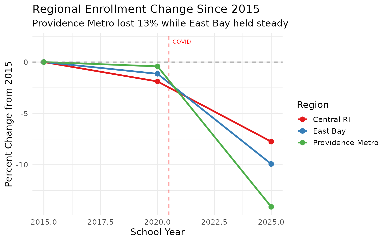
15. Providence Metro shrank 13% while East Bay held steady
The East Bay communities (Barrington, Bristol Warren) have held enrollment relatively steady while Providence Metro districts (Providence, Pawtucket, Central Falls) declined sharply since 2015.
regions <- enr_2025 |>
  filter(is_district, subgroup == "total_enrollment", grade_level == "TOTAL") |>
  mutate(region = case_when(
    district_name %in% c("Barrington", "Bristol Warren") ~ "East Bay",
    district_name %in% c("Providence", "Pawtucket", "Central Falls") ~ "Providence Metro",
    district_name %in% c("Warwick", "Cranston", "West Warwick") ~ "Central RI",
    TRUE ~ "Other"
  )) |>
  filter(region != "Other") |>
  group_by(region) |>
  summarize(total_students = sum(n_students, na.rm = TRUE), .groups = "drop")

stopifnot(nrow(regions) > 0)
regions
#> # A tibble: 3 × 2
#>   region           total_students
#>   <chr>                     <dbl>
#> 1 Central RI                21359
#> 2 East Bay                   5987
#> 3 Providence Metro          30626
print(regions)
#> # A tibble: 3 × 2
#>   region           total_students
#>   <chr>                     <dbl>
#> 1 Central RI                21359
#> 2 East Bay                   5987
#> 3 Providence Metro          30626

# Compare regional trends over time
regional_trends <- fetch_enr_multi(c(2015, 2020, 2025), use_cache = TRUE) |>
  filter(is_district, subgroup == "total_enrollment", grade_level == "TOTAL") |>
  mutate(region = case_when(
    district_name %in% c("Barrington", "Bristol Warren") ~ "East Bay",
    district_name %in% c("Providence", "Pawtucket", "Central Falls") ~ "Providence Metro",
    district_name %in% c("Warwick", "Cranston", "West Warwick") ~ "Central RI",
    TRUE ~ NA_character_
  )) |>
  filter(!is.na(region)) |>
  group_by(end_year, region) |>
  summarize(total_students = sum(n_students, na.rm = TRUE), .groups = "drop") |>
  group_by(region) |>
  mutate(pct_change = (total_students / first(total_students) - 1) * 100)

stopifnot(nrow(regional_trends) > 0)

regional_trends |>
  ggplot(aes(x = end_year, y = pct_change, color = region)) +
  geom_line(linewidth = 1.2) +
  geom_point(size = 3) +
  geom_hline(yintercept = 0, linetype = "dashed", color = "gray50") +
  geom_vline(xintercept = 2020.5, linetype = "dashed", color = "red", alpha = 0.5) +
  annotate("text", x = 2020.5, y = 2, label = "COVID", hjust = -0.2, color = "red", size = 3) +
  scale_color_brewer(palette = "Set1") +
  labs(
    title = "Regional Enrollment Change Since 2015",
    subtitle = "Providence Metro lost 13% while East Bay held steady",
    x = "School Year",
    y = "Percent Change from 2015",
    color = "Region"
  )
Summary
Rhode Island’s school enrollment data reveals:
- Post-COVID decline: The state lost 7,815 students since 2011, with most of the decline after COVID
- Providence dominance: One district serves 15% of all students but lost 3,705 since 2019
- Demographic shift: Hispanic enrollment grew from 22% to 31% since 2012
- English learner surge: LEP population tripled from 5.9% to 15.0% of enrollment
- Charter growth: Charter schools grew from 3,705 to 13,078 students (9.6% of enrollment)
- Kindergarten decline: Down 12% since 2012 with no post-COVID recovery
- Approaching minority-majority: White students hold a slim 50.3% majority
- Rising special ed: Special education rate surged from 15.8% to 18.5%
- Suburban divergence: Cranston held enrollment better than Warwick, opening a 2,184-student gap
- Newport’s struggle: Tourism economy has not prevented a 13% enrollment decline
- Regional divides: East Bay held steady while Providence Metro declined 13%
These patterns shape school funding formulas and facility planning across the Ocean State.
Data sourced from the Rhode Island Department of Education Data Center.
sessionInfo()
#> R version 4.5.2 (2025-10-31)
#> Platform: x86_64-pc-linux-gnu
#> Running under: Ubuntu 24.04.3 LTS
#>
#> Matrix products: default
#> BLAS:   /usr/lib/x86_64-linux-gnu/openblas-pthread/libblas.so.3
#> LAPACK: /usr/lib/x86_64-linux-gnu/openblas-pthread/libopenblasp-r0.3.26.so;  LAPACK version 3.12.0
#>
#> locale:
#>  [1] LC_CTYPE=C.UTF-8       LC_NUMERIC=C           LC_TIME=C.UTF-8
#>  [4] LC_COLLATE=C.UTF-8     LC_MONETARY=C.UTF-8    LC_MESSAGES=C.UTF-8
#>  [7] LC_PAPER=C.UTF-8       LC_NAME=C              LC_ADDRESS=C
#> [10] LC_TELEPHONE=C         LC_MEASUREMENT=C.UTF-8 LC_IDENTIFICATION=C
#>
#> time zone: UTC
#> tzcode source: system (glibc)
#>
#> attached base packages:
#> [1] stats     graphics  grDevices utils     datasets  methods   base
#>
#> other attached packages:
#> [1] ggplot2_4.0.2      tidyr_1.3.2        dplyr_1.2.0        rischooldata_0.1.0
#> [5] testthat_3.3.2
#>
#> loaded via a namespace (and not attached):
#>  [1] gtable_0.3.6       jsonlite_2.0.0     compiler_4.5.2     brio_1.1.5
#>  [5] tidyselect_1.2.1   jquerylib_0.1.4    systemfonts_1.3.2  scales_1.4.0
#>  [9] textshaping_1.0.5  readxl_1.4.5       yaml_2.3.12        fastmap_1.2.0
#> [13] R6_2.6.1           labeling_0.4.3     generics_0.1.4     curl_7.0.0
#> [17] knitr_1.51         forcats_1.0.1      tibble_3.3.1       desc_1.4.3
#> [21] bslib_0.10.0       pillar_1.11.1      RColorBrewer_1.1-3 rlang_1.1.7
#> [25] utf8_1.2.6         cachem_1.1.0       xfun_0.56          S7_0.2.1
#> [29] fs_1.6.7           sass_0.4.10        viridisLite_0.4.3  cli_3.6.5
#> [33] withr_3.0.2        pkgdown_2.2.0      magrittr_2.0.4     digest_0.6.39
#> [37] grid_4.5.2         rappdirs_0.3.4     lifecycle_1.0.5    vctrs_0.7.1
#> [41] evaluate_1.0.5     glue_1.8.0         cellranger_1.1.0   farver_2.1.2
#> [45] codetools_0.2-20   ragg_1.5.1         httr_1.4.8         rmarkdown_2.30
#> [49] purrr_1.2.1        tools_4.5.2        pkgconfig_2.0.3    htmltools_0.5.9