15 Insights from Alaska School Enrollment Data
Source:vignettes/enrollment_hooks.Rmd
enrollment_hooks.Rmd
library(akschooldata)
library(dplyr)
library(tidyr)
library(ggplot2)

theme_set(theme_minimal(base_size = 14))

# Get available year range from package
available <- get_available_years()
min_year <- available$min_year
max_year <- available$max_year
all_years <- min_year:max_year
This vignette explores Alaska’s public school enrollment data, surfacing key trends and patterns across 5 years of data (2021-2025).
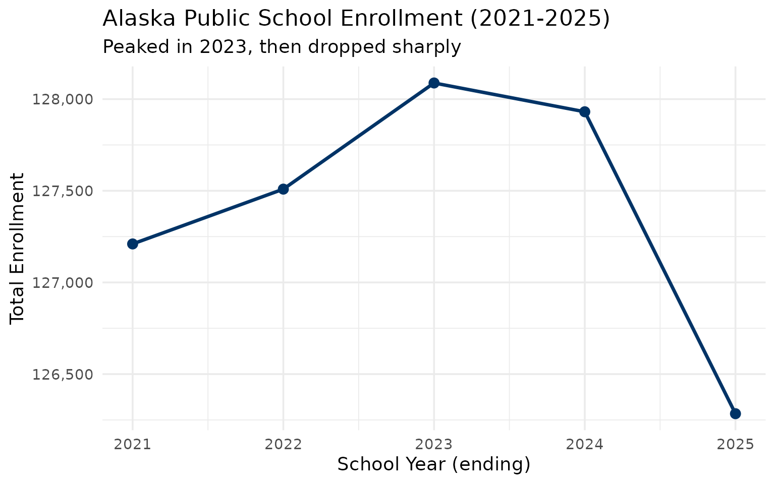
1. Alaska enrollment peaked in 2023, then dropped
Alaska’s public school enrollment rose from 127,210 in 2021 to 128,088 in 2023 before falling sharply to 126,284 in 2025–a net loss of nearly 1,000 students in five years.
enr <- fetch_enr_multi(all_years, use_cache = TRUE)

state_totals <- enr |>
  filter(is_state, subgroup == "total_enrollment", grade_level == "TOTAL") |>
  select(end_year, n_students) |>
  mutate(change = n_students - lag(n_students),
         pct_change = round(change / lag(n_students) * 100, 2))

stopifnot(nrow(state_totals) > 0)
print(state_totals)
#>   end_year n_students change pct_change
#> 1     2021     127210     NA         NA
#> 2     2022     127509    299       0.24
#> 3     2023     128088    579       0.45
#> 4     2024     127931   -157      -0.12
#> 5     2025     126284  -1647      -1.29
ggplot(state_totals, aes(x = end_year, y = n_students)) +
  geom_line(linewidth = 1.2, color = "#003366") +
  geom_point(size = 3, color = "#003366") +
  scale_y_continuous(labels = scales::comma) +
  labs(
    title = paste0("Alaska Public School Enrollment (", min_year, "-", max_year, ")"),
    subtitle = "Peaked in 2023, then dropped sharply",
    x = "School Year (ending)",
    y = "Total Enrollment"
  )
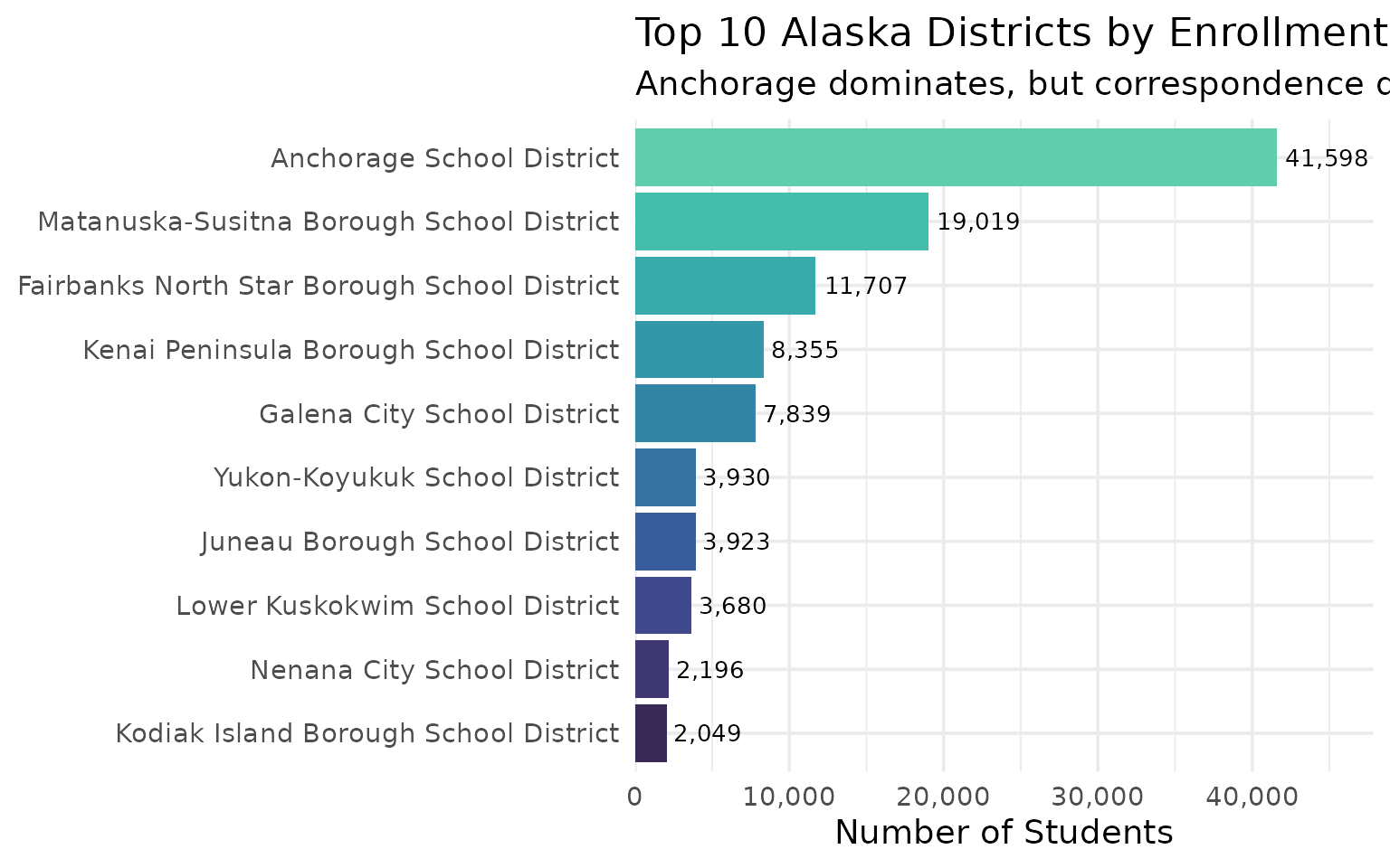
2. Anchorage is a third of the state
The Anchorage School District educates about a third of all Alaska students–41,598 out of 126,284 statewide. Galena, home to the IDEA correspondence program, is the surprising #5.
enr_latest <- fetch_enr(max_year, use_cache = TRUE)

top_districts <- enr_latest |>
  filter(is_district, subgroup == "total_enrollment", grade_level == "TOTAL") |>
  arrange(desc(n_students)) |>
  head(10) |>
  select(district_name, n_students)

stopifnot(nrow(top_districts) > 0)
print(top_districts)
#>                                   district_name n_students
#> 1                     Anchorage School District      41598
#> 2     Matanuska-Susitna Borough School District      19019
#> 3  Fairbanks North Star Borough School District      11707
#> 4       Kenai Peninsula Borough School District       8355
#> 5                   Galena City School District       7839
#> 6                 Yukon-Koyukuk School District       3930
#> 7                Juneau Borough School District       3923
#> 8               Lower Kuskokwim School District       3680
#> 9                   Nenana City School District       2196
#> 10        Kodiak Island Borough School District       2049
top_districts |>
  mutate(district_name = forcats::fct_reorder(district_name, n_students)) |>
  ggplot(aes(x = n_students, y = district_name, fill = district_name)) +
  geom_col(show.legend = FALSE) +
  geom_text(aes(label = scales::comma(n_students)), hjust = -0.1, size = 3.5) +
  scale_x_continuous(labels = scales::comma, expand = expansion(mult = c(0, 0.15))) +
  scale_fill_viridis_d(option = "mako", begin = 0.2, end = 0.8) +
  labs(
    title = paste0("Top 10 Alaska Districts by Enrollment (", max_year, ")"),
    subtitle = "Anchorage dominates, but correspondence districts rank high",
    x = "Number of Students",
    y = NULL
  )
3. Post-COVID enrollment shocks hit correspondence programs hardest
Between 2021 and 2022, the biggest enrollment drops were in correspondence-heavy districts: Hydaburg fell 24.9%, Yukon-Koyukuk 19.9%, and Galena (home to IDEA) 19.4%.
# Compare 2021 to 2022
covid_years <- 2021:2022
post_covid_enr <- fetch_enr_multi(covid_years, use_cache = TRUE)
covid_changes <- post_covid_enr |>
filter(is_district, subgroup == "total_enrollment", grade_level == "TOTAL",
end_year %in% covid_years) |>
select(district_name, end_year, n_students) |>
pivot_wider(names_from = end_year, values_from = n_students, names_prefix = "y") |>
mutate(pct_change = round((y2022 / y2021 - 1) * 100, 1)) |>
arrange(pct_change) |>
head(10) |>
select(district_name, y2021, y2022, pct_change)
stopifnot(nrow(covid_changes) > 0)
print(covid_changes)
#> # A tibble: 10 × 4
#> district_name y2021 y2022 pct_change
#> <chr> <dbl> <dbl> <dbl>
#> 1 Hydaburg City Schools 169 127 -24.9
#> 2 Yukon-Koyukuk Schools 4160 3332 -19.9
#> 3 Galena City Schools 9030 7276 -19.4
#> 4 Craig City Schools 874 713 -18.4
#> 5 Tanana Schools 30 26 -13.3
#> 6 Denali Borough Schools 1152 1003 -12.9
#> 7 Yupiit Schools 506 444 -12.3
#> 8 Nenana City Schools 1843 1633 -11.4
#> 9 Bristol Bay Borough Schools 119 106 -10.9
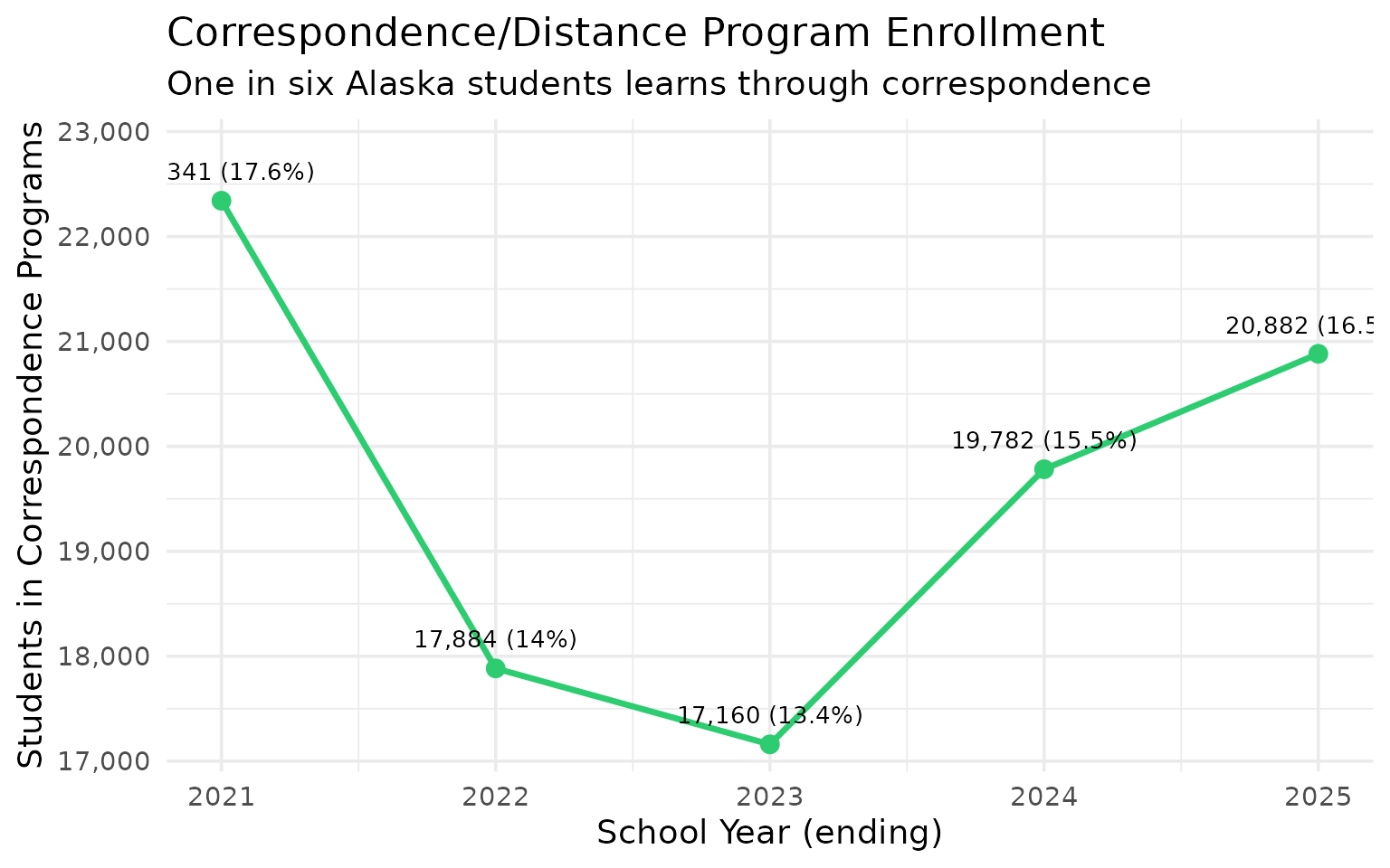
#> 10 Iditarod Area Schools 322 288 -10.64. One in six Alaska students is in a correspondence program
Correspondence and distance education schools serve over 20,000 students–about 16.5% of total statewide enrollment. These programs surged to 22,341 students in 2021, dropped during post-pandemic normalization, and are climbing again.
state_annual <- enr |>
  filter(is_state, subgroup == "total_enrollment", grade_level == "TOTAL") |>
  select(end_year, state_total = n_students)

corr_by_year <- enr |>
  filter(is_campus, subgroup == "total_enrollment", grade_level == "TOTAL") |>
  filter(grepl("IDEA|Correspondence|Distance|Central School|Raven|Cyber|Connections|PEAK|REACH|SAVE|PACE", campus_name, ignore.case = TRUE)) |>
  group_by(end_year) |>
  summarize(
    n_programs = n(),
    corr_students = sum(n_students),
    .groups = "drop"
  ) |>
  left_join(state_annual, by = "end_year") |>
  mutate(pct_of_state = round(corr_students / state_total * 100, 1))

stopifnot(nrow(corr_by_year) > 0)
print(corr_by_year)
#> # A tibble: 5 × 5
#>   end_year n_programs corr_students state_total pct_of_state
#>      <int>      <int>         <dbl>       <dbl>        <dbl>
#> 1     2021         20         22341      127210         17.6
#> 2     2022         22         17884      127509         14
#> 3     2023         22         17160      128088         13.4
#> 4     2024         23         19782      127931         15.5
#> 5     2025         24         20882      126284         16.5
ggplot(corr_by_year, aes(x = end_year, y = corr_students)) +
  geom_line(linewidth = 1.2, color = "#2ECC71") +
  geom_point(size = 3, color = "#2ECC71") +
  geom_text(aes(label = paste0(scales::comma(corr_students), " (", pct_of_state, "%)")),
            vjust = -1.2, size = 3.5) +
  scale_y_continuous(labels = scales::comma, expand = expansion(mult = c(0.05, 0.15))) +
  labs(
    title = "Correspondence/Distance Program Enrollment",
    subtitle = "One in six Alaska students learns through correspondence",
    x = "School Year (ending)",
    y = "Students in Correspondence Programs"
  )
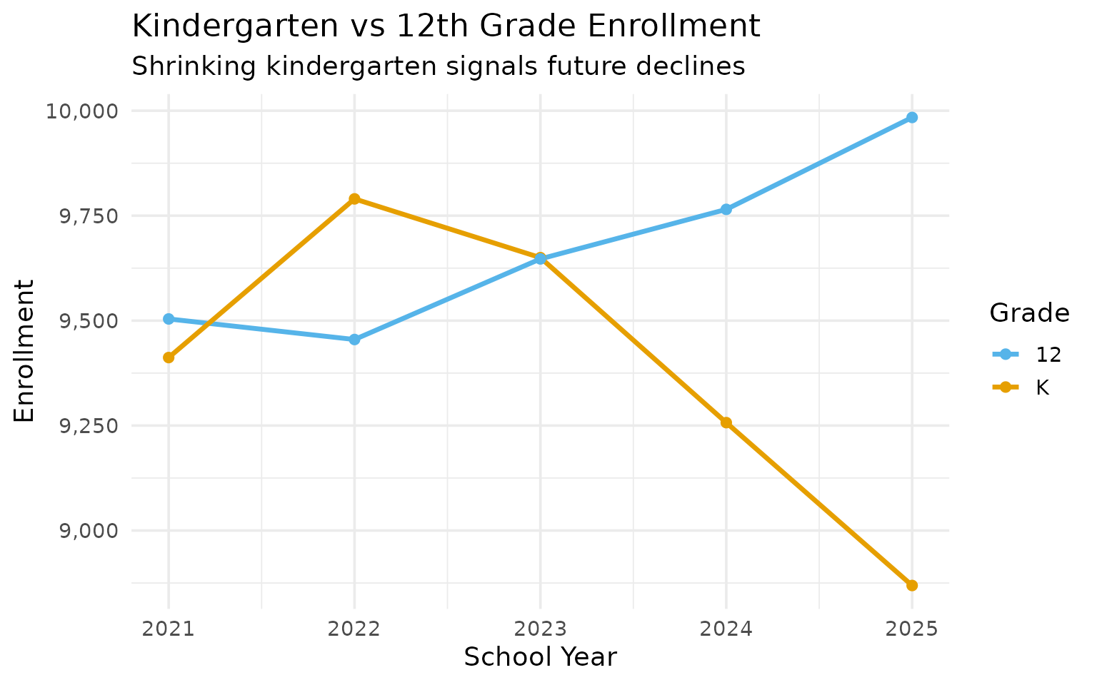
5. Kindergarten is dropping while 12th grade grows
Kindergarten enrollment fell from 9,790 in 2022 to 8,869 in 2025, while 12th grade grew from 9,455 to 9,984 over the same period. The pipeline is getting thinner at the bottom.
grade_trends <- enr |>
  filter(is_state, subgroup == "total_enrollment",
         grade_level %in% c("K", "12")) |>
  select(end_year, grade_level, n_students) |>
  pivot_wider(names_from = grade_level, values_from = n_students)

stopifnot(nrow(grade_trends) > 0)
print(grade_trends)
#> # A tibble: 5 × 3
#>   end_year     K  `12`
#>      <int> <dbl> <dbl>
#> 1     2021  9412  9504
#> 2     2022  9790  9455
#> 3     2023  9650  9647
#> 4     2024  9257  9765
#> 5     2025  8869  9984
enr |>
  filter(is_state, subgroup == "total_enrollment",
         grade_level %in% c("K", "12")) |>
  ggplot(aes(x = end_year, y = n_students, color = grade_level)) +
  geom_line(linewidth = 1.2) +
  geom_point(size = 2) +
  scale_y_continuous(labels = scales::comma) +
  scale_color_manual(values = c("K" = "#E69F00", "12" = "#56B4E9")) +
  labs(
    title = "Kindergarten vs 12th Grade Enrollment",
    subtitle = "Shrinking kindergarten signals future declines",
    x = "School Year",
    y = "Enrollment",
    color = "Grade"
  )
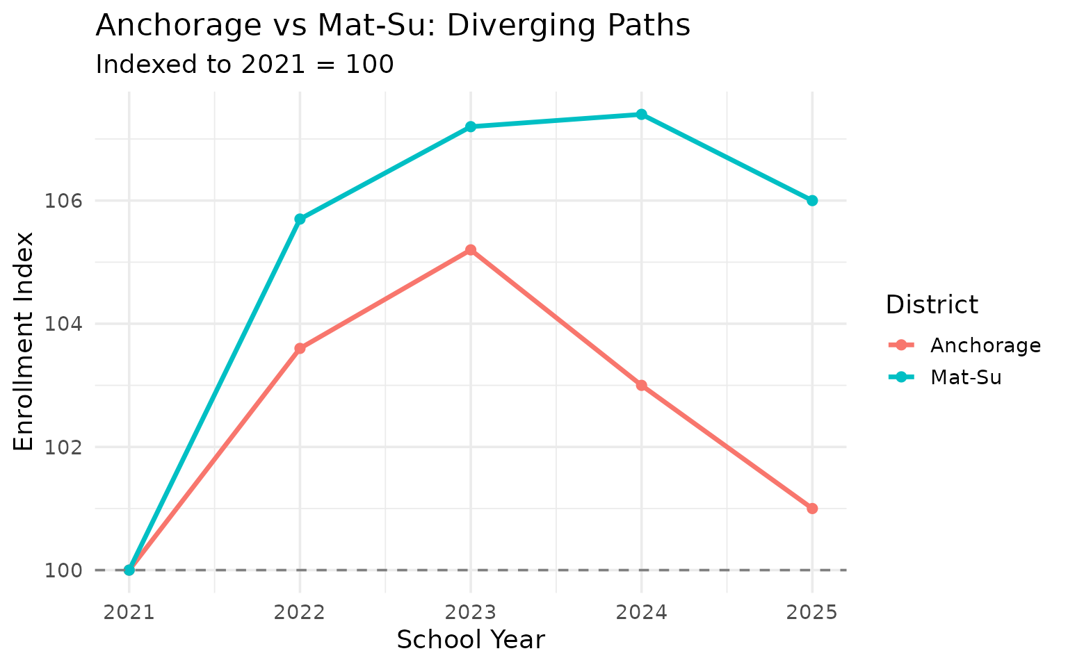
6. Mat-Su grew while Anchorage fluctuated
The Matanuska-Susitna Borough School District (Palmer/Wasilla area) grew from 17,935 to 19,019 students between 2021 and 2025, while Anchorage’s numbers rose and fell with no clear direction.
matsu <- enr |>
  filter(is_district, subgroup == "total_enrollment", grade_level == "TOTAL",
         grepl("Mat-Su|Matanuska", district_name, ignore.case = TRUE)) |>
  select(end_year, district_name, n_students)

stopifnot(nrow(matsu) > 0)
print(matsu)
#>   end_year                             district_name n_students
#> 1     2021                    Mat-Su Borough Schools      17935
#> 2     2022                    Mat-Su Borough Schools      18957
#> 3     2023                    Mat-Su Borough Schools      19225
#> 4     2024 Matanuska-Susitna Borough School District      19271
#> 5     2025 Matanuska-Susitna Borough School District      19019
enr |>
  filter(is_district, subgroup == "total_enrollment", grade_level == "TOTAL",
         grepl("Mat-Su|Matanuska|Anchorage", district_name, ignore.case = TRUE)) |>
  mutate(district_simple = case_when(
    grepl("Mat-Su|Matanuska", district_name) ~ "Mat-Su",
    grepl("Anchorage", district_name) ~ "Anchorage",
    TRUE ~ district_name
  )) |>
  group_by(district_simple) |>
  mutate(index = round(n_students / first(n_students) * 100, 1)) |>
  ggplot(aes(x = end_year, y = index, color = district_simple)) +
  geom_line(linewidth = 1.2) +
  geom_point(size = 2) +
  geom_hline(yintercept = 100, linetype = "dashed", color = "gray50") +
  labs(
    title = "Anchorage vs Mat-Su: Diverging Paths",
    subtitle = paste0("Indexed to ", min_year, " = 100"),
    x = "School Year",
    y = "Enrollment Index",
    color = "District"
  )
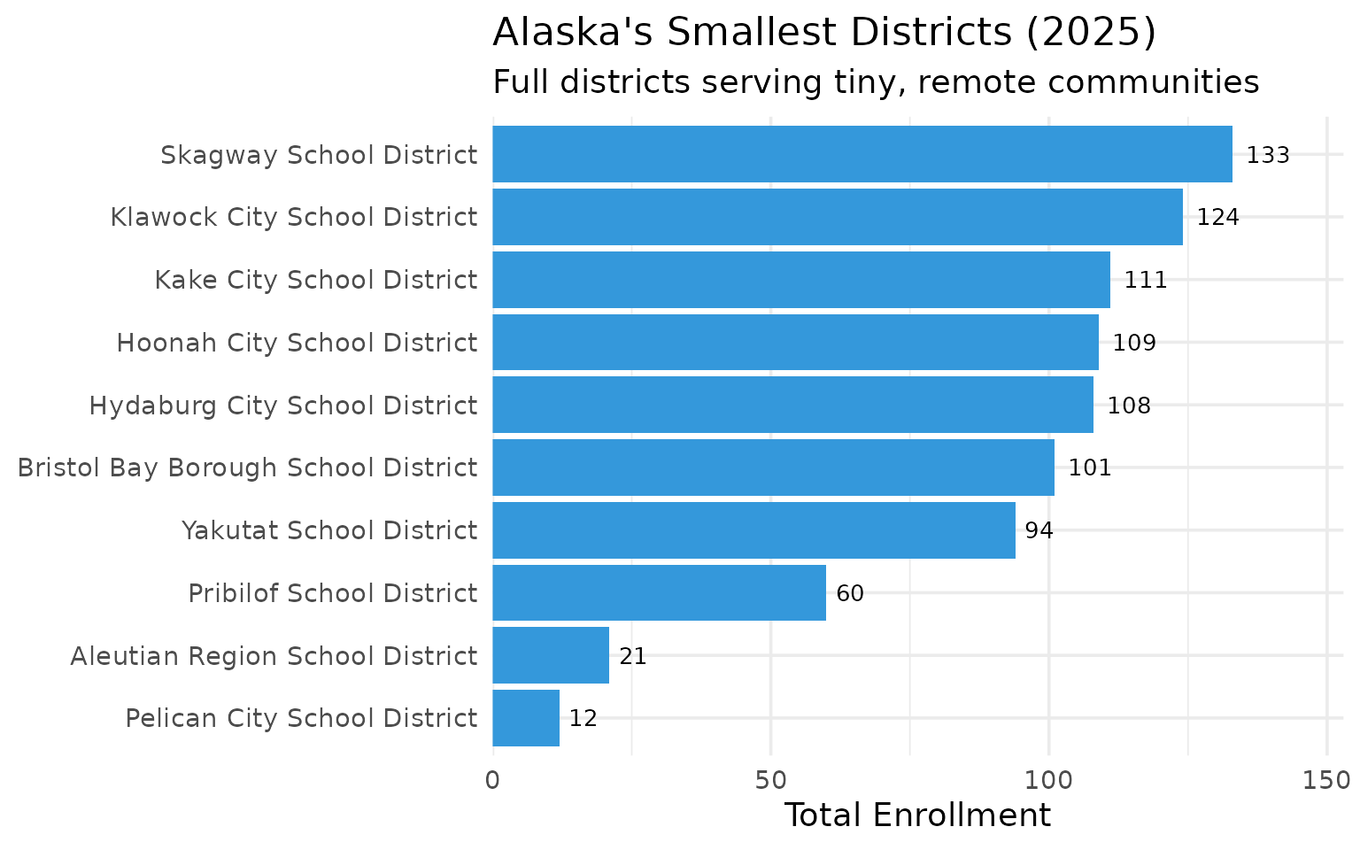
7. Fifteen districts have fewer than 200 students
Fifteen Alaska districts serve fewer than 200 students each. The smallest, Pelican City School District, has just 12 students. These tiny districts face unique challenges in America’s most remote state.
small_districts <- enr_latest |>
  filter(is_district, subgroup == "total_enrollment", grade_level == "TOTAL") |>
  filter(n_students < 200) |>
  arrange(n_students) |>
  select(district_name, n_students)

stopifnot(nrow(small_districts) > 0)
print(small_districts)
#>                             district_name n_students
#> 1            Pelican City School District         12
#> 2         Aleutian Region School District         21
#> 3                Pribilof School District         60
#> 4                 Yakutat School District         94
#> 5     Bristol Bay Borough School District        101
#> 6           Hydaburg City School District        108
#> 7             Hoonah City School District        109
#> 8               Kake City School District        111
#> 9            Klawock City School District        124
#> 10                Skagway School District        133
#> 11                Chatham School District        161
#> 12           Saint Mary's School District        161
#> 13 Aleutians East Borough School District        163
#> 14       Southeast Island School District        164
#> 15            Yukon Flats School District        171
8. The graduation pipeline leaks in rural districts
The ratio of 12th graders to 9th graders reveals where students are leaving before graduation. Nome retains just 48.5% and Southwest Region 52.8%, while urban districts like Kodiak actually gain students.
pipeline <- enr_latest |>
filter(is_district, subgroup == "total_enrollment",
grade_level %in% c("09", "12")) |>
select(district_name, grade_level, n_students) |>
pivot_wider(names_from = grade_level, values_from = n_students) |>
mutate(ratio = round(`12` / `09` * 100, 1)) |>
filter(`09` >= 50) |>
arrange(ratio) |>
head(10) |>
select(district_name, `09`, `12`, ratio)
stopifnot(nrow(pipeline) > 0)
print(pipeline)
#> # A tibble: 10 × 4
#> district_name `09` `12` ratio
#> <chr> <dbl> <dbl> <dbl>
#> 1 Nome Public Schools 68 33 48.5
#> 2 Southwest Region School District 53 28 52.8
#> 3 Delta/Greely School District 85 56 65.9
#> 4 Lower Kuskokwim School District 339 242 71.4
#> 5 Bering Strait School District 140 120 85.7
#> 6 Mount Edgecumbe 104 94 90.4
#> 7 Matanuska-Susitna Borough School District 1446 1365 94.4
#> 8 Fairbanks North Star Borough School District 846 827 97.8
#> 9 Kenai Peninsula Borough School District 673 661 98.2
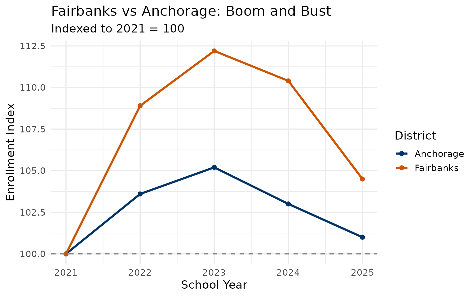
#> 10 Kodiak Island Borough School District 172 175 102.9. Anchorage and Fairbanks both grew, then contracted
Both Anchorage and Fairbanks saw enrollment rise from 2021 to 2023 before falling back. Fairbanks peaked at 112.2% of its 2021 level in 2023, then dropped to 104.5% by 2025.
major_districts <- enr |>
  filter(is_district, subgroup == "total_enrollment", grade_level == "TOTAL",
         grepl("Fairbanks|Anchorage", district_name)) |>
  mutate(district_simple = case_when(
    grepl("Anchorage", district_name) ~ "Anchorage",
    grepl("Fairbanks", district_name) ~ "Fairbanks",
    TRUE ~ district_name
  )) |>
  group_by(district_simple) |>
  mutate(index = round(n_students / first(n_students) * 100, 1)) |>
  select(end_year, district_simple, n_students, index)

stopifnot(nrow(major_districts) > 0)
print(major_districts)
#> # A tibble: 10 × 4
#> # Groups:   district_simple [2]
#>    end_year district_simple n_students index
#>       <int> <chr>                <dbl> <dbl>
#>  1     2021 Anchorage            41203  100
#>  2     2021 Fairbanks            11199  100
#>  3     2022 Anchorage            42701  104.
#>  4     2022 Fairbanks            12199  109.
#>  5     2023 Anchorage            43325  105.
#>  6     2023 Fairbanks            12568  112.
#>  7     2024 Anchorage            42431  103
#>  8     2024 Fairbanks            12365  110.
#>  9     2025 Anchorage            41598  101
#> 10     2025 Fairbanks            11707  104.
enr |>
  filter(is_district, subgroup == "total_enrollment", grade_level == "TOTAL",
         grepl("Fairbanks|Anchorage", district_name)) |>
  mutate(district_simple = case_when(
    grepl("Anchorage", district_name) ~ "Anchorage",
    grepl("Fairbanks", district_name) ~ "Fairbanks",
    TRUE ~ district_name
  )) |>
  group_by(district_simple) |>
  mutate(index = round(n_students / first(n_students) * 100, 1)) |>
  ggplot(aes(x = end_year, y = index, color = district_simple)) +
  geom_line(linewidth = 1.2) +
  geom_point(size = 2) +
  geom_hline(yintercept = 100, linetype = "dashed", color = "gray50") +
  scale_color_manual(values = c("Anchorage" = "#003366", "Fairbanks" = "#CC5500")) +
  labs(
    title = "Fairbanks vs Anchorage: Boom and Bust",
    subtitle = paste0("Indexed to ", min_year, " = 100"),
    x = "School Year",
    y = "Enrollment Index",
    color = "District"
  )
10. Alaska’s geography creates unique schools
Some Alaska schools are only accessible by plane or boat. The 10 smallest districts collectively serve fewer than 1,000 students across areas larger than many states.
smallest <- enr_latest |>
  filter(is_district, subgroup == "total_enrollment", grade_level == "TOTAL") |>
  arrange(n_students) |>
  head(10) |>
  select(district_name, n_students)

stopifnot(nrow(smallest) > 0)
print(smallest)
#>                          district_name n_students
#> 1         Pelican City School District         12
#> 2      Aleutian Region School District         21
#> 3             Pribilof School District         60
#> 4              Yakutat School District         94
#> 5  Bristol Bay Borough School District        101
#> 6        Hydaburg City School District        108
#> 7          Hoonah City School District        109
#> 8            Kake City School District        111
#> 9         Klawock City School District        124
#> 10             Skagway School District        133
11. IDEA serves more students than all but four districts
Alaska pioneered distance education out of necessity. Interior Distance Education of Alaska (IDEA) alone enrolls 7,564 students, making its parent district (Galena) the 5th largest in the state. Raven School adds another 3,603.
distance_schools <- enr_latest |>
  filter(is_campus, subgroup == "total_enrollment", grade_level == "TOTAL") |>
  filter(grepl("IDEA|Correspondence|Distance|Central School|Raven|Cyber|Connections|PEAK|REACH|SAVE|PACE", campus_name, ignore.case = TRUE)) |>
  arrange(desc(n_students)) |>
  head(10) |>
  select(district_name, campus_name, n_students)

stopifnot(nrow(distance_schools) > 0)
print(distance_schools)
#>                                district_name
#> 1                Galena City School District
#> 2              Yukon-Koyukuk School District
#> 3  Matanuska-Susitna Borough School District
#> 4                Nenana City School District
#> 5    Kenai Peninsula Borough School District
#> 6                  Anchorage School District
#> 7             Denali Borough School District
#> 8  Matanuska-Susitna Borough School District
#> 9                 Craig City School District
#> 10                 Anchorage School District
#>                                     campus_name n_students
#> 1  Interior Distance Education of Alaska (IDEA)       7564
#> 2                                  Raven School       3603
#> 3                         Mat-Su Central School       2780
#> 4              CyberLynx Correspondence Program       2002
#> 5                                   Connections       1144
#> 6      Family Partnership Correspondence School       1008
#> 7                                   Denali PEAK        854
#> 8                       Pioneer Peak Elementary        449
#> 9                           PACE Correspondence        414
#> 10                         Ravenwood Elementary        345
distance_schools |>
  mutate(campus_name = forcats::fct_reorder(campus_name, n_students)) |>
  ggplot(aes(x = n_students, y = campus_name, fill = district_name)) +
  geom_col() +
  geom_text(aes(label = scales::comma(n_students)), hjust = -0.1, size = 3.5) +
  scale_x_continuous(labels = scales::comma, expand = expansion(mult = c(0, 0.15))) +
  scale_fill_viridis_d(option = "plasma", begin = 0.2, end = 0.8) +
  labs(
    title = paste0("Top Distance/Correspondence Programs (", max_year, ")"),
    subtitle = "IDEA alone serves more students than most Alaska districts",
    x = "Number of Students",
    y = NULL,
    fill = "District"
  ) +
  theme(legend.position = "bottom")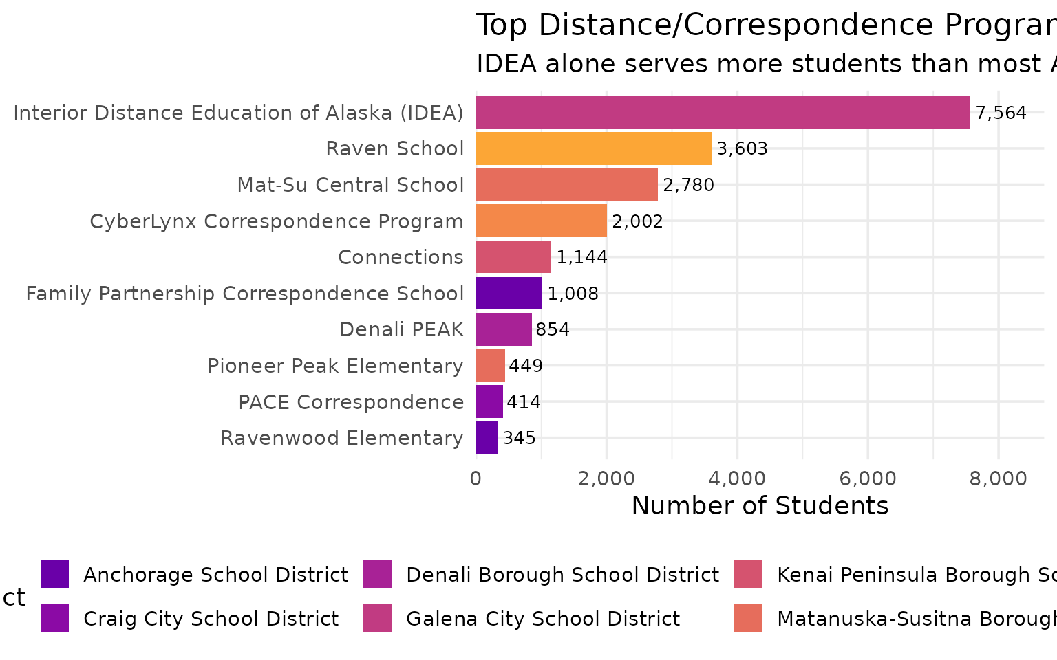
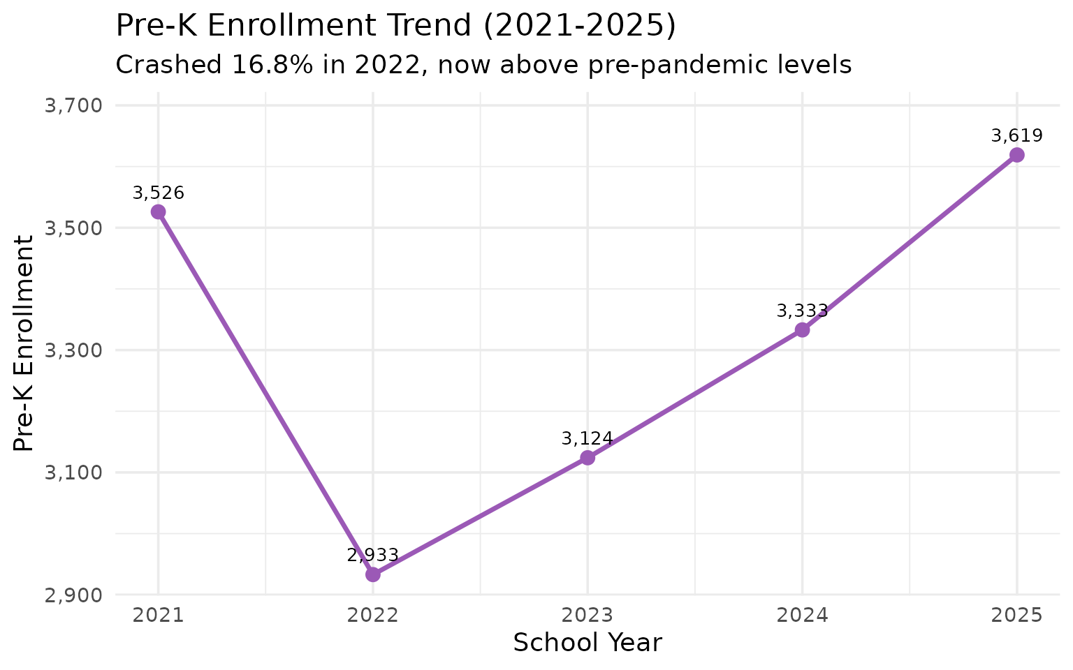
12. Pre-K crashed 16.8% in 2022, then rebounded
Pre-Kindergarten enrollment plummeted from 3,526 to 2,933 between 2021 and 2022–a 16.8% drop. It has since recovered to 3,619 in 2025, surpassing its pre-pandemic level.
prek_trend <- enr |>
  filter(is_state, subgroup == "total_enrollment", grade_level == "PK") |>
  select(end_year, n_students) |>
  mutate(change = n_students - lag(n_students),
         pct_change = round(change / lag(n_students) * 100, 1))

stopifnot(nrow(prek_trend) > 0)
print(prek_trend)
#>   end_year n_students change pct_change
#> 1     2021       3526     NA         NA
#> 2     2022       2933   -593      -16.8
#> 3     2023       3124    191        6.5
#> 4     2024       3333    209        6.7
#> 5     2025       3619    286        8.6
ggplot(prek_trend, aes(x = end_year, y = n_students)) +
  geom_line(linewidth = 1.2, color = "#9B59B6") +
  geom_point(size = 3, color = "#9B59B6") +
  geom_text(aes(label = scales::comma(n_students)), vjust = -1, size = 3.5) +
  scale_y_continuous(labels = scales::comma, expand = expansion(mult = c(0.05, 0.15))) +
  labs(
    title = paste0("Pre-K Enrollment Trend (", min_year, "-", max_year, ")"),
    subtitle = "Crashed 16.8% in 2022, now above pre-pandemic levels",
    x = "School Year",
    y = "Pre-K Enrollment"
  )
13. Elementary shrinks while high school holds steady
Elementary enrollment (K-5) fell from 58,923 to 57,282 between 2021 and 2025, while high school (9-12) actually grew from 38,168 to 39,598. Smaller incoming cohorts haven’t reached high school yet.
level_trends <- enr |>
  filter(is_state, subgroup == "total_enrollment") |>
  mutate(level = case_when(
    grade_level %in% c("K", "01", "02", "03", "04", "05") ~ "Elementary (K-5)",
    grade_level %in% c("06", "07", "08") ~ "Middle (6-8)",
    grade_level %in% c("09", "10", "11", "12") ~ "High School (9-12)",
    TRUE ~ NA_character_
  )) |>
  filter(!is.na(level)) |>
  group_by(end_year, level) |>
  summarize(n_students = sum(n_students), .groups = "drop")

stopifnot(nrow(level_trends) > 0)
print(level_trends)
#> # A tibble: 15 × 3
#>    end_year level              n_students
#>       <int> <chr>                   <dbl>
#>  1     2021 Elementary (K-5)        58923
#>  2     2021 High School (9-12)      38168
#>  3     2021 Middle (6-8)            30119
#>  4     2022 Elementary (K-5)        58895
#>  5     2022 High School (9-12)      38615
#>  6     2022 Middle (6-8)            29999
#>  7     2023 Elementary (K-5)        59000
#>  8     2023 High School (9-12)      39219
#>  9     2023 Middle (6-8)            29869
#> 10     2024 Elementary (K-5)        58554
#> 11     2024 High School (9-12)      39776
#> 12     2024 Middle (6-8)            29601
#> 13     2025 Elementary (K-5)        57282
#> 14     2025 High School (9-12)      39598
#> 15     2025 Middle (6-8)            29404
level_trends |>
  group_by(level) |>
  mutate(index = round(n_students / first(n_students) * 100, 1)) |>
  ggplot(aes(x = end_year, y = index, color = level)) +
  geom_line(linewidth = 1.2) +
  geom_point(size = 2) +
  geom_hline(yintercept = 100, linetype = "dashed", color = "gray50") +
  scale_color_manual(values = c("Elementary (K-5)" = "#E74C3C", "Middle (6-8)" = "#F39C12", "High School (9-12)" = "#27AE60")) +
  labs(
    title = "Diverging Trends by School Level",
    subtitle = paste0("Indexed to ", min_year, " = 100"),
    x = "School Year",
    y = "Enrollment Index",
    color = "Level"
  ) +
  theme(legend.position = "bottom")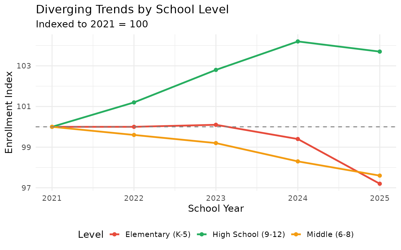
14. Twelve students, one district
Pelican City School District serves just 12 students–but under Alaska law, it still operates as a full district. Nine districts have fewer than 135 students each.
micro_districts <- enr_latest |>
  filter(is_district, subgroup == "total_enrollment", grade_level == "TOTAL") |>
  filter(n_students < 150) |>
  arrange(n_students) |>
  select(district_name, n_students) |>
  head(10)

stopifnot(nrow(micro_districts) > 0)
print(micro_districts)
#>                          district_name n_students
#> 1         Pelican City School District         12
#> 2      Aleutian Region School District         21
#> 3             Pribilof School District         60
#> 4              Yakutat School District         94
#> 5  Bristol Bay Borough School District        101
#> 6        Hydaburg City School District        108
#> 7          Hoonah City School District        109
#> 8            Kake City School District        111
#> 9         Klawock City School District        124
#> 10             Skagway School District        133
micro_districts |>
  mutate(district_name = forcats::fct_reorder(district_name, n_students)) |>
  ggplot(aes(x = n_students, y = district_name)) +
  geom_col(fill = "#3498DB") +
  geom_text(aes(label = n_students), hjust = -0.3, size = 3.5) +
  scale_x_continuous(expand = expansion(mult = c(0, 0.15))) +
  labs(
    title = paste0("Alaska's Smallest Districts (", max_year, ")"),
    subtitle = "Full districts serving tiny, remote communities",
    x = "Total Enrollment",
    y = NULL
  )
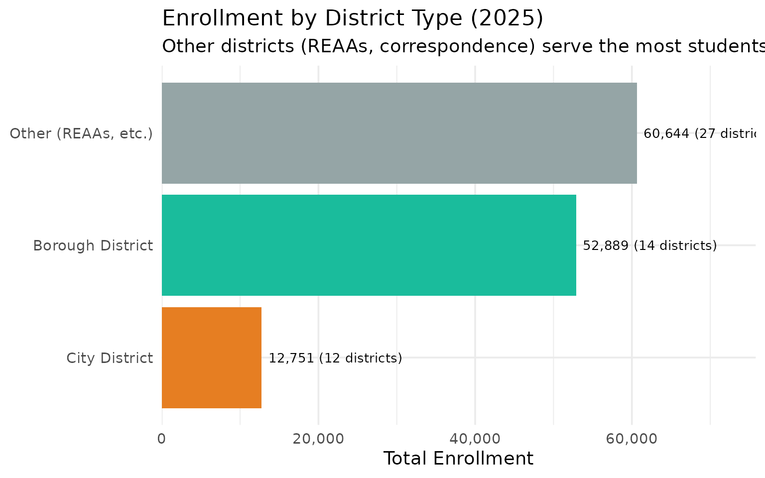
15. REAAs and other non-borough districts serve the most students
Alaska’s 27 “other” districts (REAAs, correspondence-heavy districts, and Mt. Edgecumbe) collectively serve 60,644 students–more than the 14 borough districts combined (52,889).
dist_types <- enr_latest |>
  filter(is_district, subgroup == "total_enrollment", grade_level == "TOTAL") |>
  mutate(dist_type = case_when(
    grepl("Borough", district_name) ~ "Borough District",
    grepl("City", district_name) ~ "City District",
    TRUE ~ "Other (REAAs, etc.)"
  )) |>
  group_by(dist_type) |>
  summarize(
    n_districts = n(),
    total_students = sum(n_students),
    .groups = "drop"
  ) |>
  mutate(avg_students = round(total_students / n_districts))

stopifnot(nrow(dist_types) > 0)
print(dist_types)
#> # A tibble: 3 × 4
#>   dist_type           n_districts total_students avg_students
#>   <chr>                     <int>          <dbl>        <dbl>
#> 1 Borough District             14          52889         3778
#> 2 City District                12          12751         1063
#> 3 Other (REAAs, etc.)          27          60644         2246
dist_types |>
  mutate(dist_type = forcats::fct_reorder(dist_type, total_students)) |>
  ggplot(aes(x = total_students, y = dist_type, fill = dist_type)) +
  geom_col(show.legend = FALSE) +
  geom_text(aes(label = paste0(scales::comma(total_students), " (", n_districts, " districts)")),
            hjust = -0.05, size = 3.5) +
  scale_x_continuous(labels = scales::comma, expand = expansion(mult = c(0, 0.25))) +
  scale_fill_manual(values = c("Borough District" = "#1ABC9C", "City District" = "#E67E22", "Other (REAAs, etc.)" = "#95A5A6")) +
  labs(
    title = paste0("Enrollment by District Type (", max_year, ")"),
    subtitle = "Other districts (REAAs, correspondence) serve the most students",
    x = "Total Enrollment",
    y = NULL
  )
Summary
Alaska’s school enrollment data reveals:
- Post-pandemic peak: Enrollment rose through 2023, then dropped sharply in 2024-2025
- Anchorage dominance: One district educates a third of the state
- Distance education boom: Correspondence programs serve one in six students
- Mat-Su growth: The Valley continues to attract families
- Rural resilience: Tiny bush districts persist against long odds
- Pre-K rebound: Early childhood education surpassed pre-pandemic levels
- Pipeline divergence: Elementary shrinks while high school grows
These patterns shape school funding debates and facility planning across America’s largest and most remote state.
Data sourced from the Alaska Department of Education and Early Development Data Center.
sessionInfo()
#> R version 4.5.2 (2025-10-31)
#> Platform: x86_64-pc-linux-gnu
#> Running under: Ubuntu 24.04.3 LTS
#>
#> Matrix products: default
#> BLAS:   /usr/lib/x86_64-linux-gnu/openblas-pthread/libblas.so.3
#> LAPACK: /usr/lib/x86_64-linux-gnu/openblas-pthread/libopenblasp-r0.3.26.so;  LAPACK version 3.12.0
#>
#> locale:
#>  [1] LC_CTYPE=C.UTF-8       LC_NUMERIC=C           LC_TIME=C.UTF-8
#>  [4] LC_COLLATE=C.UTF-8     LC_MONETARY=C.UTF-8    LC_MESSAGES=C.UTF-8
#>  [7] LC_PAPER=C.UTF-8       LC_NAME=C              LC_ADDRESS=C
#> [10] LC_TELEPHONE=C         LC_MEASUREMENT=C.UTF-8 LC_IDENTIFICATION=C
#>
#> time zone: UTC
#> tzcode source: system (glibc)
#>
#> attached base packages:
#> [1] stats     graphics  grDevices utils     datasets  methods   base
#>
#> other attached packages:
#> [1] ggplot2_4.0.2      tidyr_1.3.2        dplyr_1.2.0        akschooldata_0.2.0
#>
#> loaded via a namespace (and not attached):
#>  [1] gtable_0.3.6       jsonlite_2.0.0     compiler_4.5.2     tidyselect_1.2.1
#>  [5] jquerylib_0.1.4    systemfonts_1.3.2  scales_1.4.0       textshaping_1.0.5
#>  [9] readxl_1.4.5       yaml_2.3.12        fastmap_1.2.0      R6_2.6.1
#> [13] labeling_0.4.3     generics_0.1.4     curl_7.0.0         knitr_1.51
#> [17] forcats_1.0.1      tibble_3.3.1       desc_1.4.3         bslib_0.10.0
#> [21] pillar_1.11.1      RColorBrewer_1.1-3 rlang_1.1.7        utf8_1.2.6
#> [25] cachem_1.1.0       xfun_0.56          fs_1.6.7           sass_0.4.10
#> [29] S7_0.2.1           viridisLite_0.4.3  cli_3.6.5          withr_3.0.2
#> [33] pkgdown_2.2.0      magrittr_2.0.4     digest_0.6.39      grid_4.5.2
#> [37] rappdirs_0.3.4     lifecycle_1.0.5    vctrs_0.7.1        evaluate_1.0.5
#> [41] glue_1.8.0         cellranger_1.1.0   farver_2.1.2       codetools_0.2-20
#> [45] ragg_1.5.1         httr_1.4.8         rmarkdown_2.30     purrr_1.2.1
#> [49] tools_4.5.2        pkgconfig_2.0.3    htmltools_0.5.9