Connecticut Enrollment: 15 Insights from the Nutmeg State
Source:vignettes/enrollment_hooks.Rmd
enrollment_hooks.RmdThis vignette explores Connecticut public school enrollment through 15 data stories using real data from the Connecticut State Department of Education (CSDE) via the CT Open Data portal.
Data Overview
The package fetches enrollment data from two CT attendance datasets
on data.ct.gov: district-level data with 13 demographic subgroups
(he4h-bgqh) and school-level totals
(vpbj-j9a4). Available years are 2020-2023.
enr <- fetch_enr_multi(2020:2023, use_cache = TRUE)
cat("Total rows:", nrow(enr), "\n")
#> Total rows: 9071
cat("Years:", paste(sort(unique(enr$end_year)), collapse = ", "), "\n")
#> Years: 2020, 2021, 2022, 2023
cat("Subgroups:", paste(sort(unique(enr$subgroup)), collapse = ", "), "\n")
#> Subgroups: black, free_lunch, free_reduced_lunch, high_needs, hispanic, homeless, lep, other_races, reduced_lunch, special_ed, total_enrollment, white, without_high_needs
cat("Entity types:", paste(sort(unique(enr$type)), collapse = ", "), "\n")
#> Entity types: Campus, District, State
Story 1: Bridgeport leads CT’s Big 5 with 18,508 students
Connecticut’s urban core is spread across five mid-size cities rather than dominated by one megacity. Bridgeport, Waterbury, and New Haven are nearly tied at the top, each serving around 17,500-18,500 students. This decentralized pattern sets Connecticut apart from most states, where a single large district dominates.
top_districts <- enr %>%
  filter(is_district, subgroup == "total_enrollment",
         grade_level == "TOTAL", end_year == 2023) %>%
  arrange(desc(n_students)) %>%
  head(10) %>%
  select(district_name, district_id, n_students)

stopifnot(nrow(top_districts) > 0)
print(top_districts)
#>                                        district_name district_id n_students
#> 1                         Bridgeport School District     0150011      18508
#> 2                          Waterbury School District     1510011      17786
#> 3                          New Haven School District     0930011      17776
#> 4                           Stamford School District     1350011      15938
#> 5                           Hartford School District     0640011      15448
#> 6                            Danbury School District     0340011      11925
#> 7                            Norwalk School District     1030011      11326
#> 8  Connecticut Technical Education and Career System     9000016      10949
#> 9                        New Britain School District     0890011       9367
#> 10                         Fairfield School District     0510011       9279
stopifnot(nrow(top_districts) == 10)
print(summary(top_districts$n_students))
#>    Min. 1st Qu.  Median    Mean 3rd Qu.    Max.
#>    9279   11043   13686   13830   17316   18508

ggplot(top_districts,
       aes(x = reorder(district_name, n_students), y = n_students / 1000)) +
  geom_col(fill = "#2166AC") +
  coord_flip() +
  scale_y_continuous(labels = scales::comma) +
  labs(title = "Top 10 Connecticut Districts by Enrollment (2023)",
       x = NULL, y = "Students (thousands)") +
  theme_minimal(base_size = 13)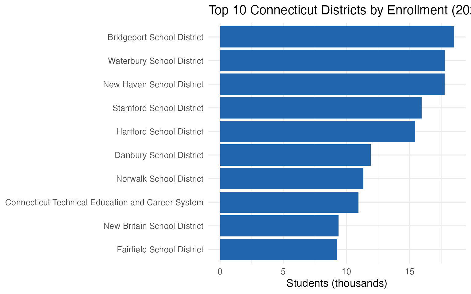
Top 10 Connecticut districts by enrollment (2023)
Story 2: Connecticut lost 14,339 students in 4 years
State enrollment fell from 508,345 in 2020 to 494,006 in 2023 – a decline of 2.8%. The steepest drop came between 2020 and 2021 (nearly 12,000 students), coinciding with pandemic-era enrollment losses. The decline continued more slowly through 2022 and 2023, with no sign of recovery.
state_trend <- enr %>%
  filter(is_state, subgroup == "total_enrollment",
         grade_level == "TOTAL") %>%
  select(end_year, n_students) %>%
  arrange(end_year) %>%
  mutate(
    change = n_students - lag(n_students),
    pct_change = round((n_students / lag(n_students) - 1) * 100, 1)
  )

stopifnot(nrow(state_trend) > 0)
print(state_trend)
#>   end_year n_students change pct_change
#> 1     2020     508345     NA         NA
#> 2     2021     496458 -11887       -2.3
#> 3     2022     495156  -1302       -0.3
#> 4     2023     494006  -1150       -0.2
stopifnot(nrow(state_trend) == 4)
print(summary(state_trend$n_students))
#>    Min. 1st Qu.  Median    Mean 3rd Qu.    Max.
#>  494006  494868  495807  498491  499430  508345

ggplot(state_trend, aes(x = end_year, y = n_students / 1000)) +
  geom_vline(xintercept = 2020.5, linetype = "dashed", color = "gray50", alpha = 0.5) +
  annotate("text", x = 2020.5, y = Inf, label = "COVID", vjust = 1.5, size = 3, color = "gray50") +
  geom_line(color = "#2166AC", linewidth = 1.2) +
  geom_point(color = "#2166AC", size = 3) +
  geom_text(aes(label = scales::comma(n_students)),
            vjust = -1.2, size = 3.5) +
  scale_x_continuous(breaks = 2020:2023) +
  scale_y_continuous(labels = scales::comma,
                     limits = c(490, 515)) +
  labs(title = "Connecticut State Enrollment (2020-2023)",
       subtitle = "Lost 14,339 students (-2.8%)",
       x = "School Year", y = "Students (thousands)") +
  theme_minimal(base_size = 13)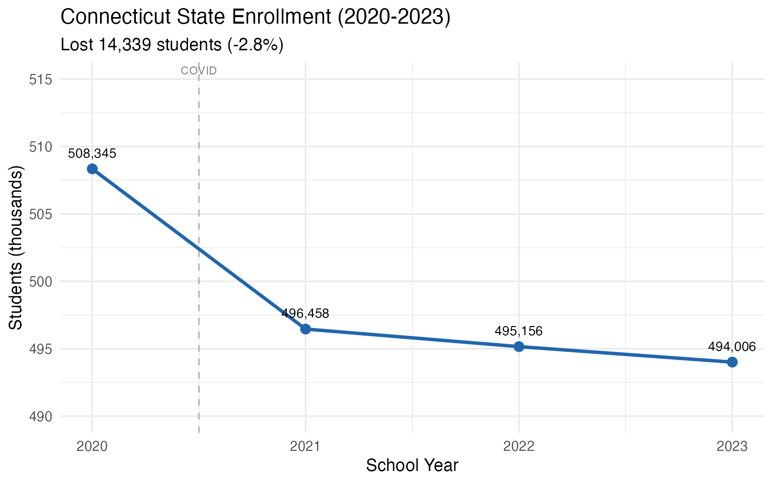
Connecticut state enrollment trend (2020-2023)
Story 3: Hartford is 58% Hispanic, 6.7% white
Hartford School District’s demographics tell the story of a majority-minority urban core surrounded by predominantly white suburbs. With 58% Hispanic students, 29.1% Black, and only 6.7% white, Hartford’s racial composition is nearly inverse of the state average.
hartford_demo <- enr %>%
  filter(is_district,
         district_name == "Hartford School District",
         end_year == 2023,
         grade_level == "TOTAL",
         subgroup %in% c("white", "black", "hispanic", "other_races",
                         "lep", "special_ed", "free_reduced_lunch",
                         "total_enrollment", "homeless")) %>%
  select(subgroup, n_students, pct) %>%
  arrange(desc(n_students))

stopifnot(nrow(hartford_demo) > 0)
print(hartford_demo)
#>             subgroup n_students         pct
#> 1   total_enrollment      15448 1.000000000
#> 2 free_reduced_lunch      12002 0.776929052
#> 3           hispanic       8957 0.579816157
#> 4              black       4490 0.290652512
#> 5                lep       3701 0.239577939
#> 6         special_ed       2993 0.193746763
#> 7              white       1034 0.066934231
#> 8        other_races        967 0.062597100
#> 9           homeless        153 0.009904195
hartford_race <- hartford_demo %>%
  filter(subgroup %in% c("white", "black", "hispanic", "other_races"))

stopifnot(nrow(hartford_race) > 0)
print(hartford_race)
#>      subgroup n_students        pct
#> 1    hispanic       8957 0.57981616
#> 2       black       4490 0.29065251
#> 3       white       1034 0.06693423
#> 4 other_races        967 0.06259710

ggplot(hartford_race,
       aes(x = reorder(subgroup, n_students), y = n_students,
           fill = subgroup)) +
  geom_col() +
  geom_text(aes(label = paste0(round(pct * 100, 1), "%")),
            hjust = -0.1, size = 3.5) +
  coord_flip() +
  scale_fill_manual(values = c("hispanic" = "#D6604D",
                                "black" = "#4393C3",
                                "white" = "#92C5DE",
                                "other_races" = "#FDDBC7"),
                    guide = "none") +
  labs(title = "Hartford School District: Race/Ethnicity (2023)",
       subtitle = "58% Hispanic, 29% Black, 6.7% white",
       x = NULL, y = "Students") +
  theme_minimal(base_size = 13)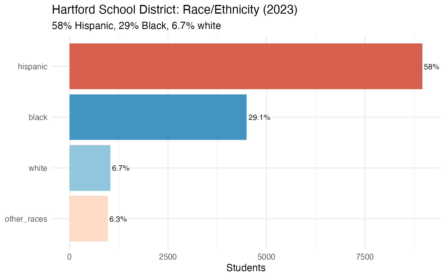
Hartford School District demographics (2023)
Story 4: Bridgeport bounced back – Hartford and New Haven didn’t
COVID hit Connecticut’s three largest cities hard, but the recovery has been uneven. Bridgeport lost 1,195 students between 2020 and 2021, then clawed most of them back by 2023. Hartford (-10.9%) and New Haven (-7.9%) kept losing students every single year, suggesting a deeper structural decline beyond the pandemic.
big_three <- enr %>%
  filter(is_district,
         district_name %in% c("Bridgeport School District",
                              "Hartford School District",
                              "New Haven School District"),
         subgroup == "total_enrollment",
         grade_level == "TOTAL") %>%
  mutate(city = gsub(" School District", "", district_name)) %>%
  select(end_year, city, n_students) %>%
  arrange(city, end_year)

stopifnot(nrow(big_three) > 0)
print(big_three)
#>    end_year       city n_students
#> 1      2020 Bridgeport      19423
#> 2      2021 Bridgeport      18228
#> 3      2022 Bridgeport      18391
#> 4      2023 Bridgeport      18508
#> 5      2020   Hartford      17344
#> 6      2021   Hartford      16371
#> 7      2022   Hartford      15790
#> 8      2023   Hartford      15448
#> 9      2020  New Haven      19307
#> 10     2021  New Haven      18586
#> 11     2022  New Haven      18001
#> 12     2023  New Haven      17776
stopifnot(nrow(big_three) == 12)
print(big_three %>% group_by(city) %>% summarize(min = min(n_students), max = max(n_students)))
#> # A tibble: 3 × 3
#>   city         min   max
#>   <chr>      <dbl> <dbl>
#> 1 Bridgeport 18228 19423
#> 2 Hartford   15448 17344
#> 3 New Haven  17776 19307

ggplot(big_three, aes(x = end_year, y = n_students / 1000, color = city)) +
  geom_vline(xintercept = 2020.5, linetype = "dashed", color = "gray50", alpha = 0.5) +
  annotate("text", x = 2020.5, y = Inf, label = "COVID", vjust = 1.5, size = 3, color = "gray50") +
  geom_line(linewidth = 1.2) +
  geom_point(size = 3) +
  scale_x_continuous(breaks = 2020:2023) +
  scale_color_manual(values = c("Bridgeport" = "#D6604D",
                                 "Hartford" = "#4393C3",
                                 "New Haven" = "#5AAE61")) +
  labs(title = "CT's Big Three: Enrollment Trends (2020-2023)",
       subtitle = "Bridgeport recovered; Hartford and New Haven kept declining",
       x = "School Year", y = "Students (thousands)",
       color = NULL) +
  theme_minimal(base_size = 13) +
  theme(legend.position = "bottom")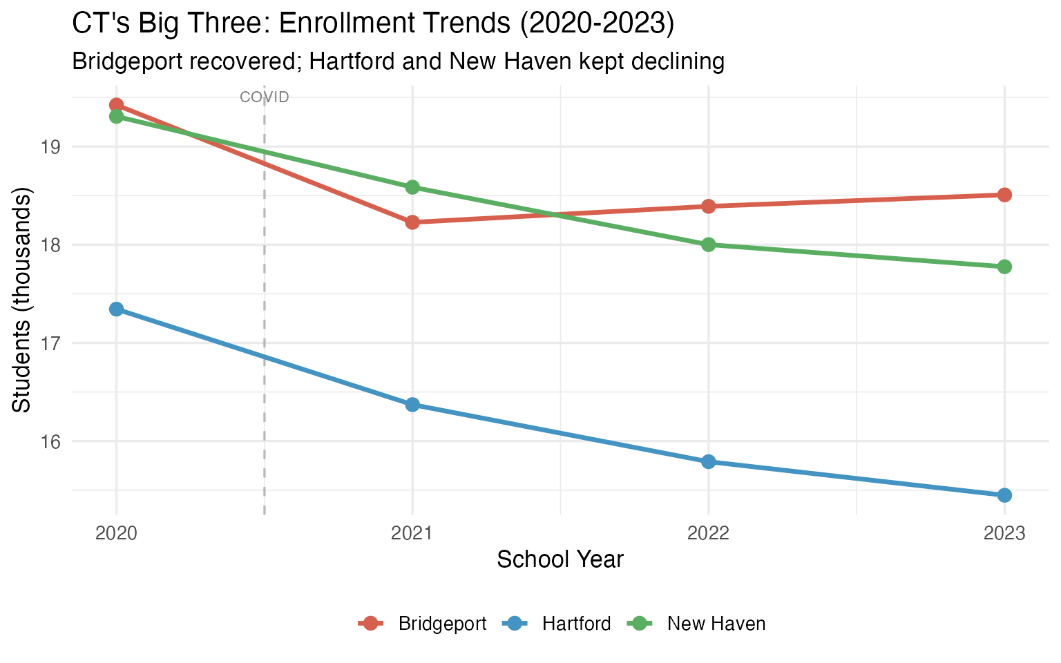
Bridgeport vs Hartford vs New Haven enrollment (2020-2023)
Story 5: CT’s 5 largest districts hold just 17% of state enrollment
Connecticut is one of the most decentralized states in the country for public education. The top 5 districts combine for just 17.2% of statewide enrollment – roughly 85,000 students out of 494,000. For comparison, many states see 25-40% of students in their top 5. With 200 districts across a small state, Connecticut’s town-by-town governance model creates extreme fragmentation.
state_total_2023 <- enr %>%
  filter(is_state, subgroup == "total_enrollment",
         grade_level == "TOTAL", end_year == 2023) %>%
  pull(n_students)

top_5 <- enr %>%
  filter(is_district, subgroup == "total_enrollment",
         grade_level == "TOTAL", end_year == 2023) %>%
  arrange(desc(n_students)) %>%
  head(5) %>%
  select(district_name, n_students) %>%
  mutate(pct_of_state = round(n_students / state_total_2023 * 100, 1))

rest_of_state <- data.frame(
  group = c("Top 5 Districts", "All Other Districts"),
  n_students = c(sum(top_5$n_students),
                 state_total_2023 - sum(top_5$n_students))
)

stopifnot(nrow(top_5) == 5)
cat("State total (2023):", scales::comma(state_total_2023), "\n")
#> State total (2023): 494,006
cat("Top 5 combined:", scales::comma(sum(top_5$n_students)), "\n")
#> Top 5 combined: 85,456
cat("Top 5 share:", round(sum(top_5$n_students) / state_total_2023 * 100, 1), "%\n\n")
#> Top 5 share: 17.3 %
print(top_5)
#>                district_name n_students pct_of_state
#> 1 Bridgeport School District      18508          3.7
#> 2  Waterbury School District      17786          3.6
#> 3  New Haven School District      17776          3.6
#> 4   Stamford School District      15938          3.2
#> 5   Hartford School District      15448          3.1
stopifnot(nrow(rest_of_state) == 2)
print(rest_of_state)
#>                 group n_students
#> 1     Top 5 Districts      85456
#> 2 All Other Districts     408550

ggplot(rest_of_state,
       aes(x = "", y = n_students / 1000, fill = group)) +
  geom_col(width = 1) +
  coord_flip() +
  scale_fill_manual(values = c("Top 5 Districts" = "#D6604D",
                                "All Other Districts" = "#92C5DE")) +
  labs(title = "CT's 5 Largest Districts: Just 17% of State Enrollment",
       subtitle = paste0("Top 5 = ", scales::comma(sum(top_5$n_students)),
                         " out of ", scales::comma(state_total_2023), " students"),
       x = NULL, y = "Students (thousands)", fill = NULL) +
  theme_minimal(base_size = 13) +
  theme(legend.position = "bottom",
        axis.text.y = element_blank())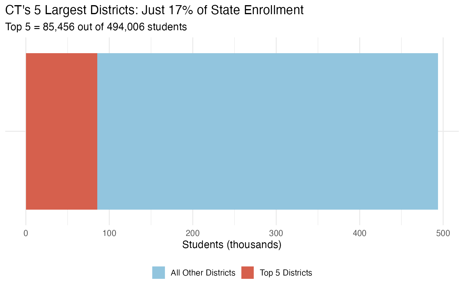
Top 5 districts’ share of Connecticut enrollment (2023)
Story 6: Hispanic enrollment crossed 30% statewide in 2023
Hispanic students grew from 26.9% of Connecticut’s public school enrollment in 2020 to 30.2% in 2023 – an increase of 12,249 students even as overall enrollment shrank. This is a significant demographic milestone: nearly one in three Connecticut public school students is now Hispanic.
hispanic_trend <- enr %>%
  filter(is_state, subgroup == "hispanic",
         grade_level == "TOTAL") %>%
  select(end_year, n_students, pct) %>%
  arrange(end_year) %>%
  mutate(pct_display = round(pct * 100, 1))

stopifnot(nrow(hispanic_trend) > 0)
print(hispanic_trend)
#>   end_year n_students       pct pct_display
#> 1     2020     136948 0.2693997        26.9
#> 2     2021     138910 0.2798021        28.0
#> 3     2022     144253 0.2913284        29.1
#> 4     2023     149197 0.3020146        30.2
stopifnot(nrow(hispanic_trend) == 4)
print(summary(hispanic_trend$pct))
#>    Min. 1st Qu.  Median    Mean 3rd Qu.    Max.
#>  0.2694  0.2772  0.2856  0.2856  0.2940  0.3020

ggplot(hispanic_trend, aes(x = end_year, y = pct * 100)) +
  geom_vline(xintercept = 2020.5, linetype = "dashed", color = "gray50", alpha = 0.5) +
  annotate("text", x = 2020.5, y = Inf, label = "COVID", vjust = 1.5, size = 3, color = "gray50") +
  geom_line(color = "#D6604D", linewidth = 1.2) +
  geom_point(color = "#D6604D", size = 3) +
  geom_text(aes(label = paste0(round(pct * 100, 1), "%")),
            vjust = -1.2, size = 3.5) +
  geom_hline(yintercept = 30, linetype = "dashed", color = "gray50") +
  scale_x_continuous(breaks = 2020:2023) +
  scale_y_continuous(limits = c(25, 33)) +
  labs(title = "Hispanic Students Crossed 30% of CT Enrollment in 2023",
       subtitle = "From 136,948 (26.9%) in 2020 to 149,197 (30.2%) in 2023",
       x = "School Year", y = "Percent of Total Enrollment") +
  theme_minimal(base_size = 13)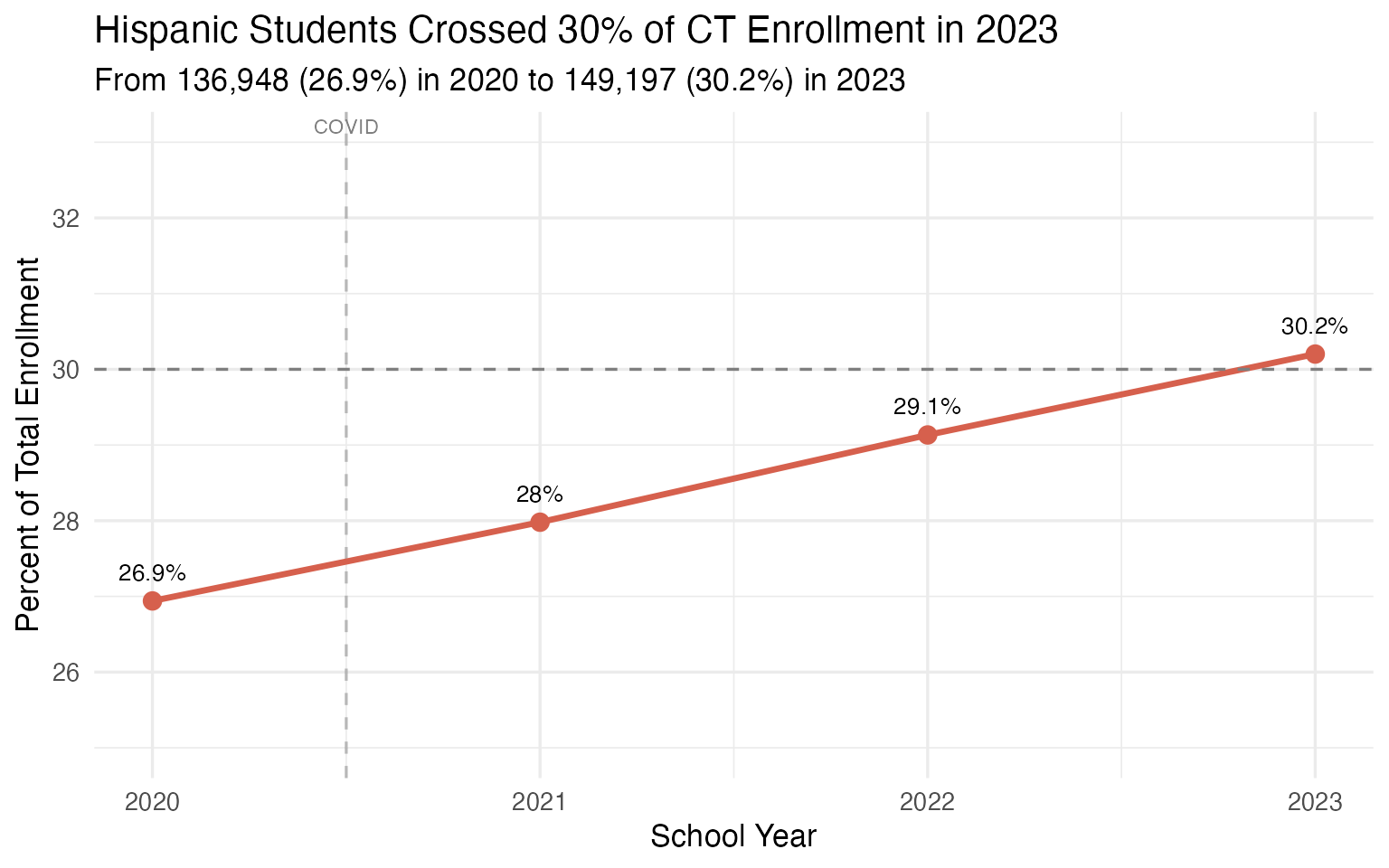
Hispanic enrollment share in Connecticut (2020-2023)
Story 7: 1 in 3 students in Danbury and Windham are English learners
English learner (LEP) concentration varies enormously across Connecticut. In Danbury and Windham, roughly a third of students are English learners. Compare that to affluent suburbs where the rate is below 2%. This hyper-concentration creates staffing and resource challenges in just a handful of districts.
lep_districts <- enr %>%
  filter(is_district, subgroup == "lep",
         grade_level == "TOTAL", end_year == 2023) %>%
  arrange(desc(pct)) %>%
  head(10) %>%
  mutate(city = gsub(" School District", "", district_name),
         pct_display = round(pct * 100, 1)) %>%
  select(city, district_name, n_students, pct_display)

stopifnot(nrow(lep_districts) > 0)
print(lep_districts)
#>                                               city
#> 1                                          Danbury
#> 2                                          Windham
#> 3                                       New London
#> 4                                       Bridgeport
#> 5                                         Hartford
#> 6                                          Norwich
#> 7                                        New Haven
#> 8  Interdistrict School for Arts and Comm District
#> 9                             Side By Side Charter
#> 10                                         Norwalk
#>                                      district_name n_students pct_display
#> 1                          Danbury School District       3936        33.0
#> 2                          Windham School District        978        32.9
#> 3                       New London School District        758        26.6
#> 4                       Bridgeport School District       4781        25.8
#> 5                         Hartford School District       3701        24.0
#> 6                          Norwich School District        690        21.5
#> 7                        New Haven School District       3735        21.0
#> 8  Interdistrict School for Arts and Comm District         56        20.9
#> 9             Side By Side Charter School District         38        19.5
#> 10                         Norwalk School District       2144        18.9
stopifnot(nrow(lep_districts) == 10)
print(summary(lep_districts$pct_display))
#>    Min. 1st Qu.  Median    Mean 3rd Qu.    Max.
#>   18.90   20.93   22.75   24.41   26.40   33.00

ggplot(lep_districts,
       aes(x = reorder(city, pct_display), y = pct_display)) +
  geom_col(fill = "#5AAE61") +
  geom_text(aes(label = paste0(pct_display, "%")),
            hjust = -0.1, size = 3.5) +
  coord_flip() +
  scale_y_continuous(limits = c(0, max(lep_districts$pct_display) * 1.15)) +
  labs(title = "Top 10 CT Districts by English Learner Rate (2023)",
       subtitle = "Danbury and Windham: ~1 in 3 students",
       x = NULL, y = "Percent LEP") +
  theme_minimal(base_size = 13)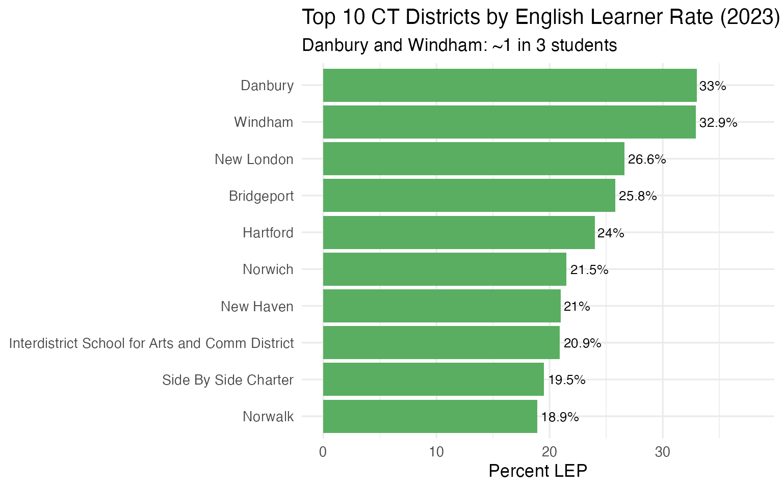
Top 10 CT districts by English learner percentage (2023)
Story 8: 84% of New London students qualify for free/reduced lunch
Free and reduced-price lunch eligibility is the most widely used proxy for student poverty, and the variation across Connecticut is staggering. In New London, 84% of students qualify. In nearby affluent communities, the rate drops below 5%. This gap captures Connecticut’s well-documented wealth inequality.
frl_districts <- enr %>%
  filter(is_district, subgroup == "free_reduced_lunch",
         grade_level == "TOTAL", end_year == 2023) %>%
  arrange(desc(pct)) %>%
  head(10) %>%
  mutate(city = gsub(" School District", "", district_name),
         pct_display = round(pct * 100, 1)) %>%
  select(city, district_name, n_students, pct_display)

stopifnot(nrow(frl_districts) > 0)
print(frl_districts)
#>                                             city
#> 1                                     New London
#> 2          Booker T. Washington Academy District
#> 3                              Highville Charter
#> 4                   Elm City College Preparatory
#> 5                                       Hartford
#> 6                       Amistad Academy District
#> 7                                     Unified #2
#> 8                                     Bridgeport
#> 9                                        Meriden
#> 10 Achievement First Bridgeport Academy District
#>                                    district_name n_students pct_display
#> 1                     New London School District       2393        84.0
#> 2          Booker T. Washington Academy District        338        81.1
#> 3              Highville Charter School District        317        78.9
#> 4   Elm City College Preparatory School District        594        78.5
#> 5                       Hartford School District      12002        77.7
#> 6                       Amistad Academy District        846        77.3
#> 7                     Unified School District #2         53        76.8
#> 8                     Bridgeport School District      14197        76.7
#> 9                        Meriden School District       6371        74.6
#> 10 Achievement First Bridgeport Academy District        774        73.8
stopifnot(nrow(frl_districts) == 10)
print(summary(frl_districts$pct_display))
#>    Min. 1st Qu.  Median    Mean 3rd Qu.    Max.
#>   73.80   76.72   77.50   77.94   78.80   84.00

ggplot(frl_districts,
       aes(x = reorder(city, pct_display), y = pct_display)) +
  geom_col(fill = "#B2182B") +
  geom_text(aes(label = paste0(pct_display, "%")),
            hjust = -0.1, size = 3.5) +
  coord_flip() +
  scale_y_continuous(limits = c(0, 100)) +
  labs(title = "Top 10 CT Districts by Free/Reduced Lunch Rate (2023)",
       subtitle = "New London leads at 84%",
       x = NULL, y = "Percent FRL") +
  theme_minimal(base_size = 13)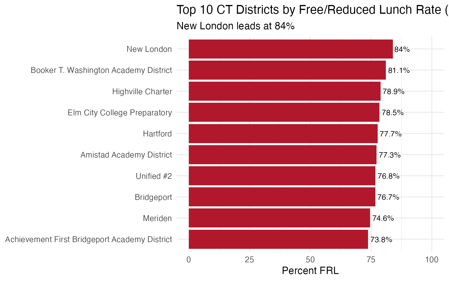
Top 10 CT districts by free/reduced lunch rate (2023)
Story 9: Special education co-ops serve mostly IEP students
Connecticut has several cooperative educational service districts that specialize in serving students with disabilities. Unified School District #1, Cooperative Educational Services, and Area Cooperative Educational Services all have special education rates above 40% – because their primary mission is to provide specialized services that individual towns cannot offer alone.
sped_districts <- enr %>%
  filter(is_district, subgroup == "special_ed",
         grade_level == "TOTAL", end_year == 2023) %>%
  arrange(desc(pct)) %>%
  head(10) %>%
  mutate(pct_display = round(pct * 100, 1)) %>%
  select(district_name, n_students, pct_display)

stopifnot(nrow(sped_districts) > 0)
print(sped_districts)
#>                                                         district_name
#> 1                                          Unified School District #1
#> 2                                    Cooperative Educational Services
#> 3                               Area Cooperative Educational Services
#> 4  Eastern Connecticut Regional Educational Service Center (EASTCONN)
#> 5                                               Explorations District
#> 6                                  Common Ground High School District
#> 7                                            Scotland School District
#> 8                                         Regional School District 07
#> 9                                            Hartland School District
#> 10                                        Regional School District 13
#>    n_students pct_display
#> 1          74        60.2
#> 2         333        50.1
#> 3         734        42.6
#> 4         141        36.2
#> 5          25        30.5
#> 6          58        28.6
#> 7          20        25.6
#> 8         200        22.6
#> 9          24        22.0
#> 10        298        21.9
stopifnot(nrow(sped_districts) == 10)
print(summary(sped_districts$pct_display))
#>    Min. 1st Qu.  Median    Mean 3rd Qu.    Max.
#>   21.90   23.35   29.55   34.03   41.00   60.20

ggplot(sped_districts,
       aes(x = reorder(district_name, pct_display), y = pct_display)) +
  geom_col(fill = "#7570B3") +
  geom_text(aes(label = paste0(pct_display, "%")),
            hjust = -0.1, size = 3.5) +
  coord_flip() +
  scale_y_continuous(limits = c(0, max(sped_districts$pct_display) * 1.15)) +
  labs(title = "Top 10 CT Districts by Special Education Rate (2023)",
       subtitle = "Co-ops and unified districts dominate the list",
       x = NULL, y = "Percent Special Ed") +
  theme_minimal(base_size = 13)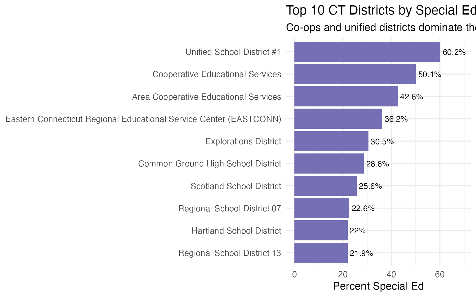
Top 10 CT districts by special education rate (2023)
Story 10: Student homelessness dropped 39% in 4 years
Connecticut identified 3,916 students experiencing homelessness in 2020 but only 2,385 in 2023 – a 39% decline. The dip in 2021 (3,110) may reflect undercounting during remote learning, and the bump in 2022 (3,645) coincides with pandemic-era housing instability. The 2023 drop to the lowest count in the series is notable.
homeless_trend <- enr %>%
  filter(is_state, subgroup == "homeless",
         grade_level == "TOTAL") %>%
  select(end_year, n_students, pct) %>%
  arrange(end_year) %>%
  mutate(pct_display = round(pct * 100, 2))

stopifnot(nrow(homeless_trend) > 0)
print(homeless_trend)
#>   end_year n_students         pct pct_display
#> 1     2020       3916 0.007703430        0.77
#> 2     2021       3110 0.006264377        0.63
#> 3     2022       3645 0.007361316        0.74
#> 4     2023       2385 0.004827877        0.48
stopifnot(nrow(homeless_trend) == 4)
print(summary(homeless_trend$n_students))
#>    Min. 1st Qu.  Median    Mean 3rd Qu.    Max.
#>    2385    2929    3378    3264    3713    3916

ggplot(homeless_trend, aes(x = end_year, y = n_students)) +
  geom_vline(xintercept = 2020.5, linetype = "dashed", color = "gray50", alpha = 0.5) +
  annotate("text", x = 2020.5, y = Inf, label = "COVID", vjust = 1.5, size = 3, color = "gray50") +
  geom_line(color = "#B2182B", linewidth = 1.2) +
  geom_point(color = "#B2182B", size = 3) +
  geom_text(aes(label = scales::comma(n_students)),
            vjust = -1.2, size = 3.5) +
  scale_x_continuous(breaks = 2020:2023) +
  scale_y_continuous(labels = scales::comma,
                     limits = c(2000, 4500)) +
  labs(title = "Students Experiencing Homelessness in CT (2020-2023)",
       subtitle = "Down 39%: from 3,916 to 2,385",
       x = "School Year", y = "Homeless Students") +
  theme_minimal(base_size = 13)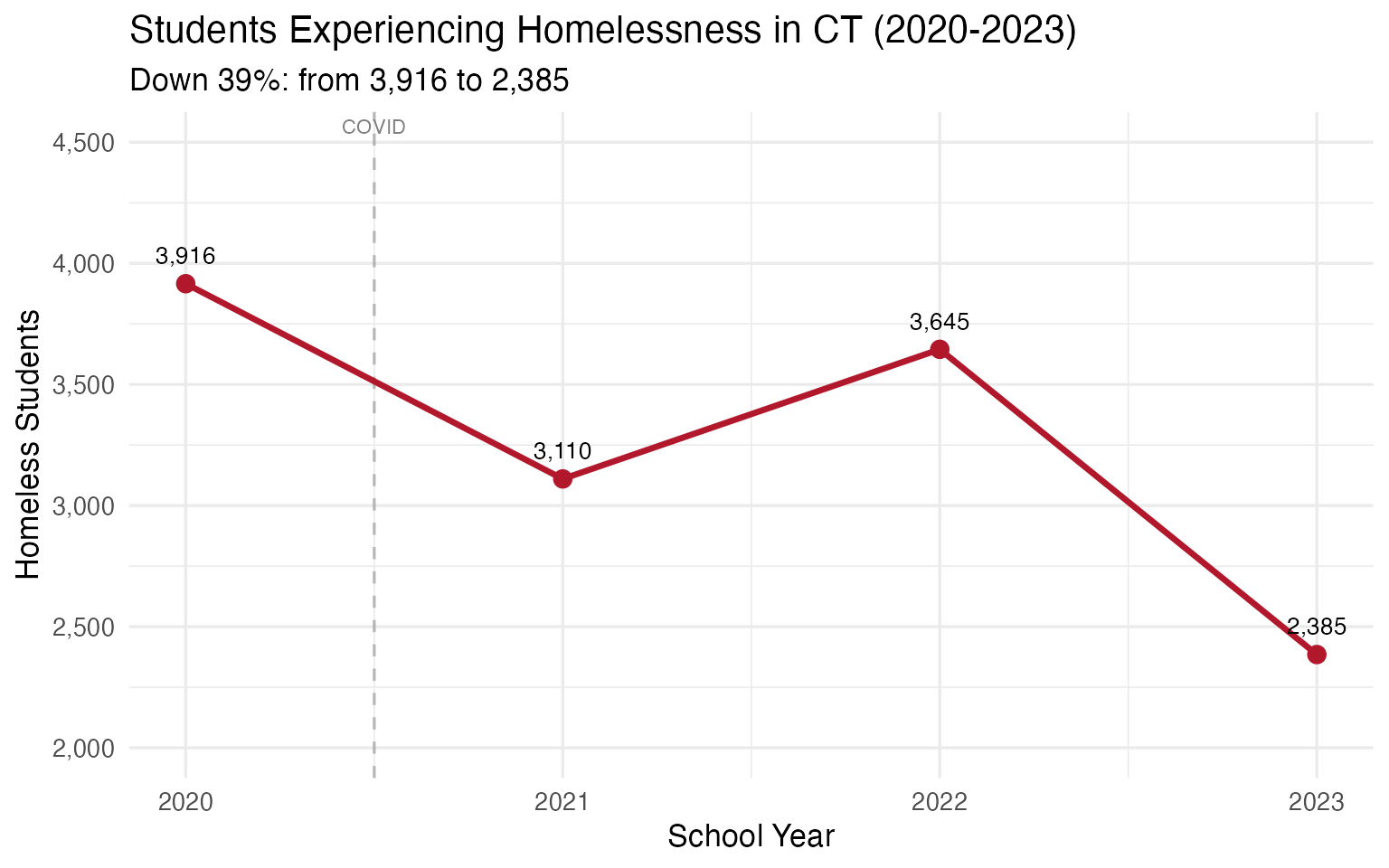
Students experiencing homelessness in Connecticut (2020-2023)
Story 11: Half of CT students are classified “high needs”
Connecticut’s “high needs” designation – which includes students who are economically disadvantaged, English learners, or receiving special education services – covers just over half the student body. The rate dropped slightly from 52.5% in 2020 to 50.8% in 2023, mainly because the denominator shrank faster than the high-needs population.
high_needs_trend <- enr %>%
  filter(is_state,
         subgroup %in% c("high_needs", "without_high_needs"),
         grade_level == "TOTAL") %>%
  select(end_year, subgroup, n_students, pct) %>%
  arrange(end_year, desc(n_students))

stopifnot(nrow(high_needs_trend) > 0)
print(high_needs_trend)
#>   end_year           subgroup n_students       pct
#> 1     2020         high_needs     266735 0.5247125
#> 2     2020 without_high_needs     241610 0.4752875
#> 3     2021         high_needs     255883 0.5154172
#> 4     2021 without_high_needs     240575 0.4845828
#> 5     2022         high_needs     259420 0.5239157
#> 6     2022 without_high_needs     235736 0.4760843
#> 7     2023         high_needs     250820 0.5077266
#> 8     2023 without_high_needs     243186 0.4922734
hn_pct <- high_needs_trend %>%
  filter(subgroup == "high_needs") %>%
  mutate(pct_display = round(pct * 100, 1))

stopifnot(nrow(hn_pct) > 0)
print(hn_pct)
#>   end_year   subgroup n_students       pct pct_display
#> 1     2020 high_needs     266735 0.5247125        52.5
#> 2     2021 high_needs     255883 0.5154172        51.5
#> 3     2022 high_needs     259420 0.5239157        52.4
#> 4     2023 high_needs     250820 0.5077266        50.8

ggplot(high_needs_trend,
       aes(x = end_year, y = n_students / 1000, fill = subgroup)) +
  geom_vline(xintercept = 2020.5, linetype = "dashed", color = "gray50", alpha = 0.5) +
  annotate("text", x = 2020.5, y = Inf, label = "COVID", vjust = 1.5, size = 3, color = "gray50") +
  geom_area(alpha = 0.8) +
  scale_fill_manual(values = c("high_needs" = "#D6604D",
                                "without_high_needs" = "#92C5DE"),
                    labels = c("High Needs", "Not High Needs")) +
  scale_x_continuous(breaks = 2020:2023) +
  scale_y_continuous(labels = scales::comma) +
  labs(title = "Half of CT Students Classified as 'High Needs'",
       subtitle = "52.5% in 2020, 50.8% in 2023",
       x = "School Year", y = "Students (thousands)",
       fill = NULL) +
  theme_minimal(base_size = 13) +
  theme(legend.position = "bottom")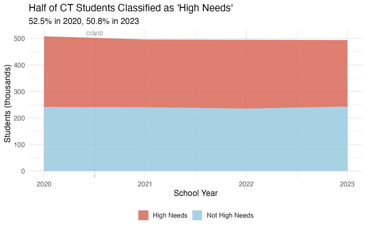
High needs vs non-high-needs students in Connecticut (2020-2023)
Story 12: Danbury High is CT’s largest school at 3,497 students
At the school level, Danbury High School towers over the rest with 3,497 students – over 800 more than the next largest school. The top 10 schools are almost all comprehensive high schools in mid-size cities and affluent suburbs.
top_schools <- enr %>%
  filter(is_campus, subgroup == "total_enrollment",
         grade_level == "TOTAL", end_year == 2023) %>%
  arrange(desc(n_students)) %>%
  head(10) %>%
  mutate(city = gsub(" School District", "", district_name)) %>%
  select(campus_name, city, n_students)

stopifnot(nrow(top_schools) > 0)
print(top_schools)
#>                campus_name                          city n_students
#> 1      Danbury High School                       Danbury       3497
#> 2    Greenwich High School                     Greenwich       2651
#> 3     Westhill High School                      Stamford       2229
#> 4  New Britain High School                   New Britain       2210
#> 5     Trumbull High School                      Trumbull       2128
#> 6     Stamford High School                      Stamford       2028
#> 7     Norwich Free Academy Norwich Free Academy District       2013
#> 8  Southington High School                   Southington       1930
#> 9  Glastonbury High School                   Glastonbury       1803
#> 10  West Haven High School                    West Haven       1742
stopifnot(nrow(top_schools) == 10)
print(summary(top_schools$n_students))
#>    Min. 1st Qu.  Median    Mean 3rd Qu.    Max.
#>    1742    1951    2078    2223    2224    3497

ggplot(top_schools,
       aes(x = reorder(campus_name, n_students), y = n_students)) +
  geom_col(fill = "#2166AC") +
  geom_text(aes(label = scales::comma(n_students)),
            hjust = -0.1, size = 3.2) +
  coord_flip() +
  scale_y_continuous(limits = c(0, max(top_schools$n_students) * 1.15),
                     labels = scales::comma) +
  labs(title = "Top 10 Connecticut Schools by Enrollment (2023)",
       subtitle = "Danbury High leads with 3,497 students",
       x = NULL, y = "Students") +
  theme_minimal(base_size = 13)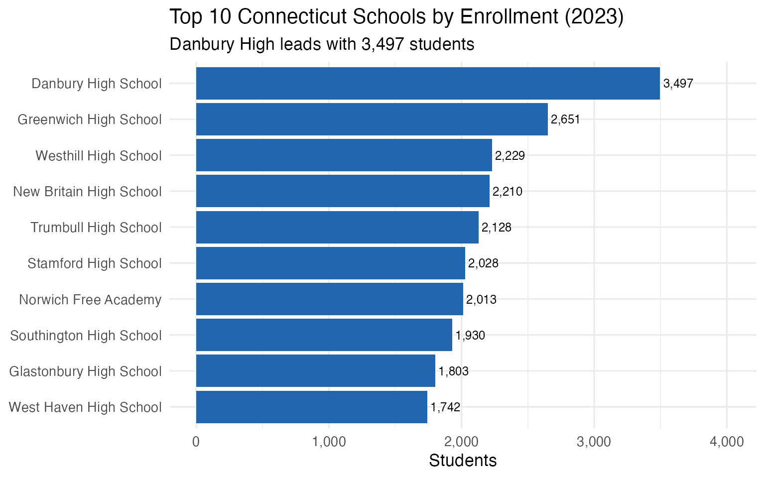
Top 10 Connecticut schools by enrollment (2023)
Story 13: 8 charter schools serve just 3,131 students – 0.6% of the state
Connecticut has one of the smallest charter school sectors in the country. Just 8 charter schools enroll a combined 3,131 students – 0.6% of statewide enrollment. The largest, Great Oaks Charter School, has only 608 students. Compare this to states like Arizona or Florida where charter schools serve 15-20% of students.
charters <- enr %>%
  filter(is_charter, subgroup == "total_enrollment",
         grade_level == "TOTAL", end_year == 2023) %>%
  arrange(desc(n_students)) %>%
  select(campus_name, district_name, n_students)

charter_total <- sum(charters$n_students)
charter_pct <- round(charter_total / state_total_2023 * 100, 1)

stopifnot(nrow(charters) > 0)
cat("Charter schools:", nrow(charters), "\n")
#> Charter schools: 8
cat("Total charter students:", scales::comma(charter_total), "\n")
#> Total charter students: 3,131
cat("Share of state:", charter_pct, "%\n\n")
#> Share of state: 0.6 %
print(charters)
#>                              campus_name
#> 1              Great Oaks Charter School
#> 2 Stamford Charter School for Excellence
#> 3      Charter Oak International Academy
#> 4               Highville Charter School
#> 5          Park City Prep Charter School
#> 6          Integrated Day Charter School
#> 7              Brass City Charter School
#> 8            Side By Side Charter School
#>                                     district_name n_students
#> 1              Great Oaks Charter School District        608
#> 2 Stamford Charter School for Excellence District        463
#> 3                   West Hartford School District        445
#> 4               Highville Charter School District        402
#> 5          Park City Prep Charter School District        372
#> 6          Integrated Day Charter School District        325
#> 7              Brass City Charter School District        321
#> 8            Side By Side Charter School District        195
stopifnot(nrow(charters) > 0)
print(summary(charters$n_students))
#>    Min. 1st Qu.  Median    Mean 3rd Qu.    Max.
#>   195.0   324.0   387.0   391.4   449.5   608.0

ggplot(charters,
       aes(x = reorder(campus_name, n_students), y = n_students)) +
  geom_col(fill = "#E08214") +
  geom_text(aes(label = scales::comma(n_students)),
            hjust = -0.1, size = 3.5) +
  coord_flip() +
  scale_y_continuous(limits = c(0, max(charters$n_students) * 1.2),
                     labels = scales::comma) +
  labs(title = "Connecticut Charter Schools by Enrollment (2023)",
       subtitle = paste0(nrow(charters), " schools, ",
                         scales::comma(charter_total),
                         " students (", charter_pct, "% of state)"),
       x = NULL, y = "Students") +
  theme_minimal(base_size = 13)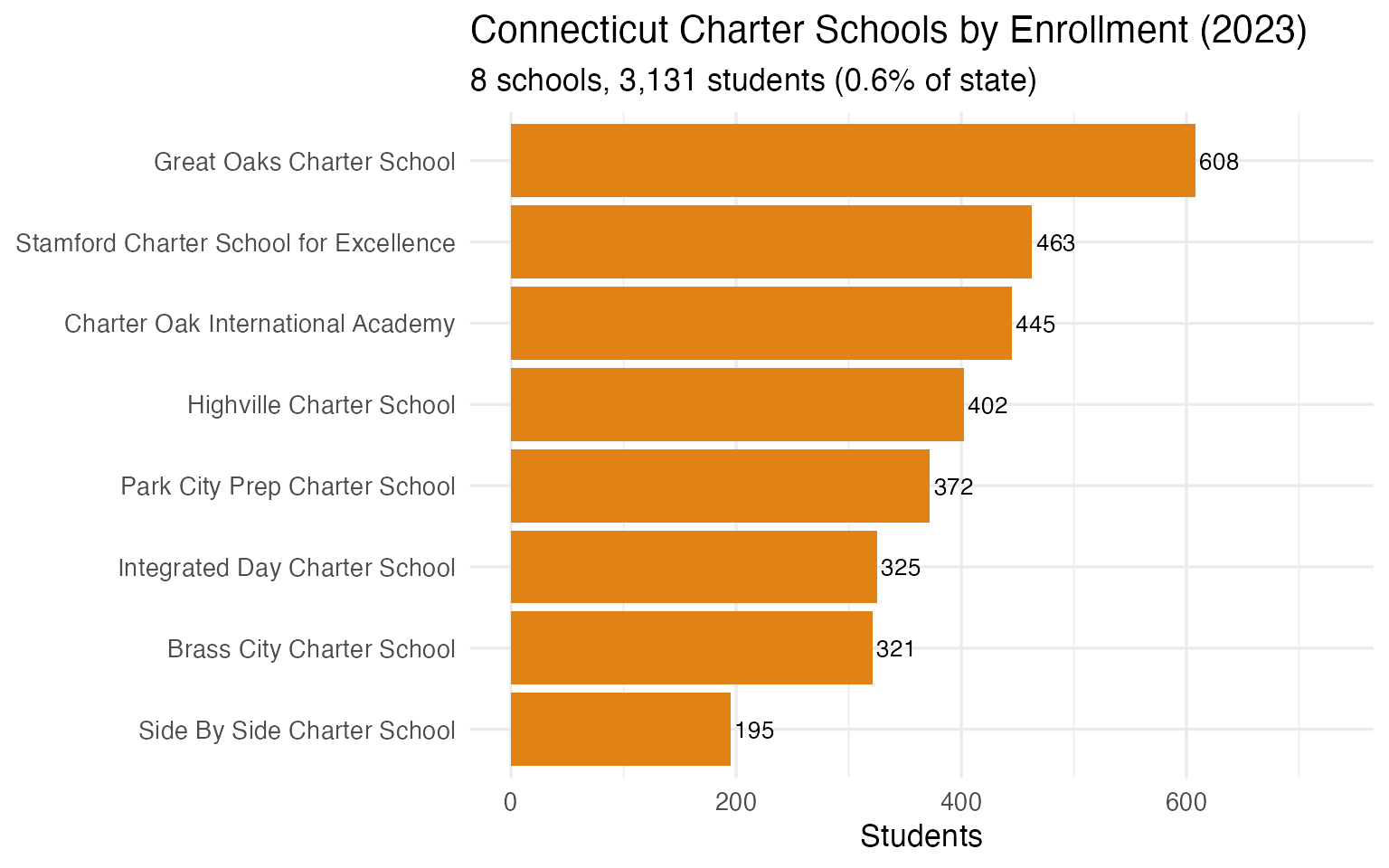
Connecticut charter schools by enrollment (2023)
Story 14: Union School District has just 48 students
On the other end of the spectrum, Connecticut’s smallest districts are remarkably tiny. Union School District enrolls just 48 students – an entire K-8 district smaller than most individual classrooms. These micro-districts reflect Connecticut’s hyper-local governance model where even the smallest towns operate independent school systems.
smallest <- enr %>%
  filter(is_district, subgroup == "total_enrollment",
         grade_level == "TOTAL", end_year == 2023,
         n_students > 0) %>%
  arrange(n_students) %>%
  head(10) %>%
  select(district_name, district_id, n_students)

stopifnot(nrow(smallest) > 0)
print(smallest)
#>                 district_name district_id n_students
#> 1       Union School District     1450011         48
#> 2     Norfolk School District     0980011         58
#> 3     Hampton School District     0630011         60
#> 4  Unified School District #2     3470015         69
#> 5   Colebrook School District     0290011         72
#> 6      Canaan School District     0210011         74
#> 7    Scotland School District     1230011         78
#> 8       Explorations District     2720013         82
#> 9    Cornwall School District     0310011         93
#> 10     Sharon School District     1250011        100
stopifnot(nrow(smallest) == 10)
print(summary(smallest$n_students))
#>    Min. 1st Qu.  Median    Mean 3rd Qu.    Max.
#>   48.00   62.25   73.00   73.40   81.00  100.00

ggplot(smallest,
       aes(x = reorder(district_name, -n_students), y = n_students)) +
  geom_col(fill = "#4393C3") +
  geom_text(aes(label = n_students), vjust = -0.5, size = 3.5) +
  coord_flip() +
  labs(title = "Smallest 10 Connecticut Districts by Enrollment (2023)",
       subtitle = "Union School District: just 48 students",
       x = NULL, y = "Students") +
  theme_minimal(base_size = 13)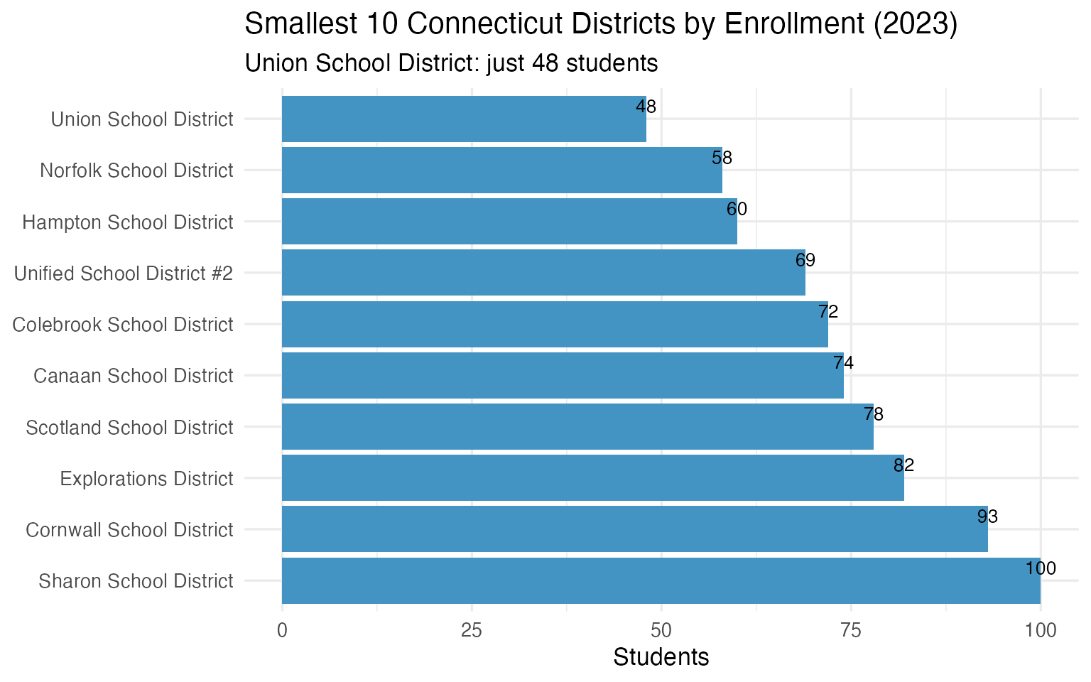
Smallest 10 Connecticut districts by enrollment (2023)
Story 15: “Other races” grew from 9.3% to 9.9% – a proxy for diversification
Connecticut’s attendance data lumps Asian, Native American, Pacific Islander, and Multiracial students into a single “other races” category. This group grew from 9.3% (47,263 students) in 2020 to 9.9% (49,090) in 2023. The steady growth suggests increasing racial diversity beyond the traditional Black-White-Hispanic categories that dominate Connecticut’s demographic conversation.
other_trend <- enr %>%
  filter(is_state, subgroup == "other_races",
         grade_level == "TOTAL") %>%
  select(end_year, n_students, pct) %>%
  arrange(end_year) %>%
  mutate(pct_display = round(pct * 100, 1))

stopifnot(nrow(other_trend) > 0)
print(other_trend)
#>   end_year n_students        pct pct_display
#> 1     2020      47263 0.09297426         9.3
#> 2     2021      47471 0.09561937         9.6
#> 3     2022      48371 0.09768841         9.8
#> 4     2023      49090 0.09937126         9.9
stopifnot(nrow(other_trend) == 4)
print(summary(other_trend$pct))
#>    Min. 1st Qu.  Median    Mean 3rd Qu.    Max.
#> 0.09297 0.09496 0.09665 0.09641 0.09811 0.09937

ggplot(other_trend, aes(x = end_year, y = pct * 100)) +
  geom_vline(xintercept = 2020.5, linetype = "dashed", color = "gray50", alpha = 0.5) +
  annotate("text", x = 2020.5, y = Inf, label = "COVID", vjust = 1.5, size = 3, color = "gray50") +
  geom_line(color = "#7570B3", linewidth = 1.2) +
  geom_point(color = "#7570B3", size = 3) +
  geom_text(aes(label = paste0(round(pct * 100, 1), "%")),
            vjust = -1.2, size = 3.5) +
  scale_x_continuous(breaks = 2020:2023) +
  scale_y_continuous(limits = c(8.5, 10.5)) +
  labs(title = "'Other Races' Share of CT Enrollment (2020-2023)",
       subtitle = "Asian, Native American, Pacific Islander, and Multiracial combined",
       x = "School Year", y = "Percent of Total Enrollment") +
  theme_minimal(base_size = 13)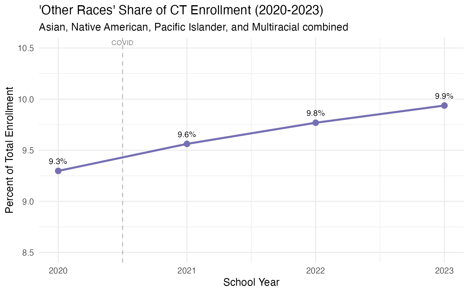
Other races enrollment share in Connecticut (2020-2023)
Session Info
sessionInfo()
#> R version 4.5.0 (2025-04-11)
#> Platform: aarch64-apple-darwin22.6.0
#> Running under: macOS 26.1
#>
#> Matrix products: default
#> BLAS:   /opt/homebrew/Cellar/openblas/0.3.30/lib/libopenblasp-r0.3.30.dylib
#> LAPACK: /opt/homebrew/Cellar/r/4.5.0/lib/R/lib/libRlapack.dylib;  LAPACK version 3.12.1
#>
#> locale:
#> [1] C.UTF-8/C.UTF-8/C.UTF-8/C/C.UTF-8/C.UTF-8
#>
#> time zone: America/New_York
#> tzcode source: internal
#>
#> attached base packages:
#> [1] stats     graphics  grDevices utils     datasets  methods   base
#>
#> other attached packages:
#> [1] forcats_1.0.1      tidyr_1.3.2        ggplot2_4.0.1      dplyr_1.2.0
#> [5] ctschooldata_0.1.0 testthat_3.3.1
#>
#> loaded via a namespace (and not attached):
#>  [1] gtable_0.3.6       jsonlite_2.0.0     compiler_4.5.0     brio_1.1.5
#>  [5] tidyselect_1.2.1   jquerylib_0.1.4    systemfonts_1.3.1  scales_1.4.0
#>  [9] textshaping_1.0.4  yaml_2.3.12        fastmap_1.2.0      R6_2.6.1
#> [13] labeling_0.4.3     generics_0.1.4     knitr_1.51         htmlwidgets_1.6.4
#> [17] tibble_3.3.1       desc_1.4.3         bslib_0.9.0        pillar_1.11.1
#> [21] RColorBrewer_1.1-3 rlang_1.1.7        utf8_1.2.6         cachem_1.1.0
#> [25] xfun_0.55          fs_1.6.6           sass_0.4.10        S7_0.2.1
#> [29] otel_0.2.0         cli_3.6.5          withr_3.0.2        pkgdown_2.2.0
#> [33] magrittr_2.0.4     digest_0.6.39      grid_4.5.0         rappdirs_0.3.4
#> [37] lifecycle_1.0.5    vctrs_0.7.1        evaluate_1.0.5     glue_1.8.0
#> [41] farver_2.1.2       codetools_0.2-20   ragg_1.5.0         purrr_1.2.1
#> [45] rmarkdown_2.30     tools_4.5.0        pkgconfig_2.0.3    htmltools_0.5.9