theme_readme <- function() {
  theme_minimal(base_size = 14) +
    theme(
      plot.title = element_text(face = "bold", size = 16),
      plot.subtitle = element_text(color = "gray40"),
      panel.grid.minor = element_blank(),
      legend.position = "bottom"
    )
}

colors <- c("total" = "#2C3E50", "growth" = "#27AE60", "decline" = "#E74C3C",
            "district1" = "#3498DB", "district2" = "#F39C12", "district3" = "#9B59B6",
            "district4" = "#1ABC9C", "district5" = "#E67E22")
# Get available years
years <- get_available_years()
if (is.list(years)) {
  max_year <- years$max_year
  min_year <- years$min_year
} else {
  max_year <- max(years)
  min_year <- min(years)
}

# Fetch data for various time spans
enr_all <- fetch_enr_multi(2002:max_year, use_cache = TRUE)
enr_decade <- fetch_enr_multi((max_year - 14):max_year, use_cache = TRUE)
enr_recent <- fetch_enr_multi((max_year - 9):max_year, use_cache = TRUE)
enr_current <- fetch_enr(max_year, use_cache = TRUE)
1. Idaho’s enrollment grew 28% in 24 years
Idaho is one of the fastest-growing states in America. Public school enrollment has surged since 2002 while many states are shrinking.
state_trend <- enr_all %>%
  filter(is_state, grade_level == "TOTAL", subgroup == "total_enrollment")
stopifnot(nrow(state_trend) > 0)

# Compute growth dynamically
first_yr <- state_trend %>% filter(end_year == min(end_year))
last_yr <- state_trend %>% filter(end_year == max(end_year))
growth <- last_yr$n_students - first_yr$n_students
pct_growth <- round((last_yr$n_students / first_yr$n_students - 1) * 100, 1)
yr_span <- max(state_trend$end_year) - min(state_trend$end_year)

state_trend %>% select(end_year, n_students)
#>    end_year n_students
#> 1      2002   246184.0
#> 2      2003   248660.0
#> 3      2004   250774.0
#> 4      2005   255980.0
#> 5      2006   262294.0
#> 6      2007   267630.0
#> 7      2008   272212.0
#> 8      2009   275113.0
#> 9      2010   278796.0
#> 10     2011   281632.0
#> 11     2012   281817.0
#> 12     2013   287620.0
#> 13     2014   289433.5
#> 14     2015   291198.0
#> 15     2016   294859.0
#> 16     2017   298765.0
#> 17     2018   302689.0
#> 18     2019   307228.0
#> 19     2020   311991.0
#> 20     2021   310653.0
#> 21     2022   316159.0
#> 22     2023   318979.0
#> 23     2024   318660.0
#> 24     2025   318067.0
#> 25     2026   314097.0
cat("Growth:", format(growth, big.mark = ","), "students (",
    pct_growth, "%) over", yr_span, "years\n")
#> Growth: 67,913 students ( 27.6 %) over 24 years

ggplot(state_trend, aes(x = end_year, y = n_students)) +
  geom_line(linewidth = 1.5, color = colors["total"]) +
  geom_point(size = 3, color = colors["total"]) +
  scale_y_continuous(labels = comma, limits = c(0, NA)) +
  labs(title = "Idaho Public School Enrollment",
       subtitle = paste0("Added ", format(growth, big.mark = ","),
                        " students since 2002 (+", pct_growth, "%)"),
       x = "School Year", y = "Students") +
  theme_readme()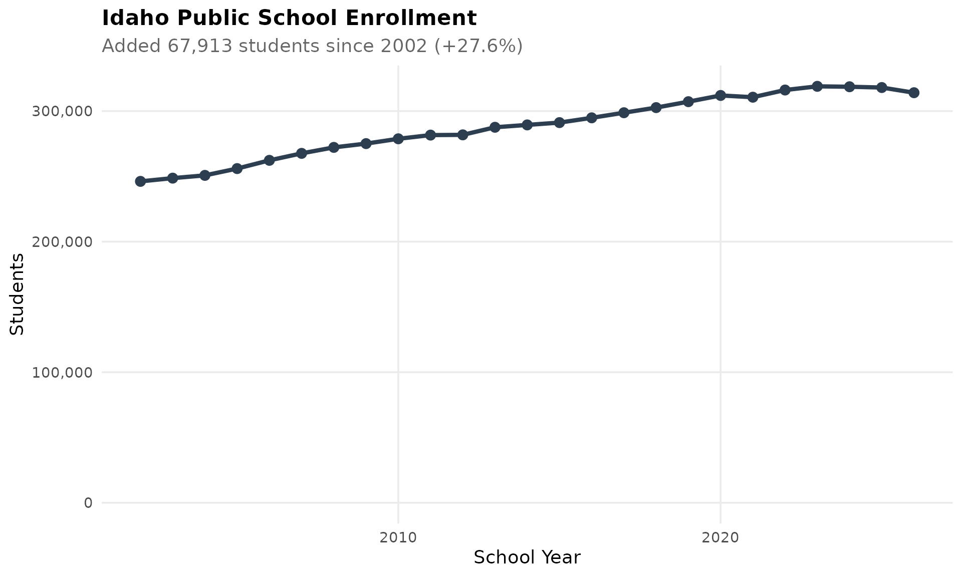
2. West Ada is Idaho’s school giant
West Ada School District in suburban Boise (Meridian/Eagle area) serves nearly 38,000 students - 75% larger than Boise itself. It’s the largest district in the state and still growing.
top_10 <- enr_current %>%
  filter(is_district, grade_level == "TOTAL", subgroup == "total_enrollment") %>%
  arrange(desc(n_students)) %>%
  head(10)
stopifnot(nrow(top_10) > 0)

# Compute ratio dynamically
west_ada <- top_10$n_students[1]
boise <- top_10$n_students[top_10$district_name == "BOISE INDEPENDENT DISTRICT"]
ratio_pct <- round((west_ada / boise - 1) * 100)

top_10 %>% select(district_name, n_students)
#>                          district_name n_students
#> 1                    WEST ADA DISTRICT      37919
#> 2           BOISE INDEPENDENT DISTRICT      21717
#> 3            BONNEVILLE JOINT DISTRICT      13511
#> 4                NAMPA SCHOOL DISTRICT      12473
#> 5                   POCATELLO DISTRICT      11437
#> 6             VALLIVUE SCHOOL DISTRICT      10700
#> 7                 IDAHO FALLS DISTRICT       9751
#> 8               COEUR D ALENE DISTRICT       9680
#> 9                  TWIN FALLS DISTRICT       8774
#> 10 IDAHO HOME LEARNING ACADEMY CHARTER       7504

ggplot(top_10, aes(x = reorder(district_name, n_students), y = n_students)) +
  geom_col(fill = colors["total"]) +
  coord_flip() +
  scale_y_continuous(labels = comma) +
  labs(title = "Idaho's Largest School Districts",
       subtitle = paste0("West Ada serves ", ratio_pct, "% more students than Boise"),
       x = "", y = "Students") +
  theme_readme()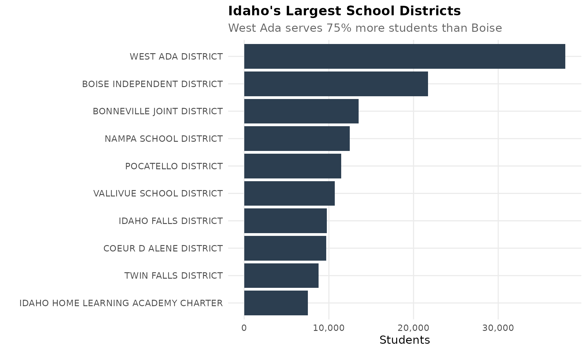
3. The Treasure Valley boom
Eagle, Kuna, Star, and Middleton are among the fastest-growing communities in America. These districts around Boise have doubled or tripled enrollment in 15 years as families flee California.
treasure_valley <- c("WEST ADA DISTRICT", "KUNA JOINT DISTRICT", "MIDDLETON DISTRICT")
tv_trend <- enr_decade %>%
  filter(is_district,
         grepl(paste(treasure_valley, collapse = "|"), district_name),
         subgroup == "total_enrollment", grade_level == "TOTAL")
stopifnot(nrow(tv_trend) > 0)
tv_trend %>% select(end_year, district_name, n_students)
#>    end_year       district_name n_students
#> 1      2012   WEST ADA DISTRICT      35188
#> 2      2012 KUNA JOINT DISTRICT       4983
#> 3      2012  MIDDLETON DISTRICT       3219
#> 4      2013   WEST ADA DISTRICT      35939
#> 5      2013 KUNA JOINT DISTRICT       5073
#> 6      2013  MIDDLETON DISTRICT       3362
#> 7      2014   WEST ADA DISTRICT      36111
#> 8      2014 KUNA JOINT DISTRICT       5102
#> 9      2014  MIDDLETON DISTRICT       3633
#> 10     2015   WEST ADA DISTRICT      36471
#> 11     2015 KUNA JOINT DISTRICT       5220
#> 12     2015  MIDDLETON DISTRICT       3768
#> 13     2016   WEST ADA DISTRICT      37366
#> 14     2016 KUNA JOINT DISTRICT       5283
#> 15     2016  MIDDLETON DISTRICT       3874
#> 16     2017   WEST ADA DISTRICT      38097
#> 17     2017 KUNA JOINT DISTRICT       5342
#> 18     2017  MIDDLETON DISTRICT       3920
#> 19     2018   WEST ADA DISTRICT      38907
#> 20     2018 KUNA JOINT DISTRICT       5397
#> 21     2018  MIDDLETON DISTRICT       4031
#> 22     2019   WEST ADA DISTRICT      39507
#> 23     2019 KUNA JOINT DISTRICT       5386
#> 24     2019  MIDDLETON DISTRICT       4086
#> 25     2020   WEST ADA DISTRICT      40326
#> 26     2020 KUNA JOINT DISTRICT       5618
#> 27     2020  MIDDLETON DISTRICT       4066
#> 28     2021   WEST ADA DISTRICT      37729
#> 29     2021 KUNA JOINT DISTRICT       5415
#> 30     2021  MIDDLETON DISTRICT       3912
#> 31     2022   WEST ADA DISTRICT      39027
#> 32     2022 KUNA JOINT DISTRICT       5738
#> 33     2022  MIDDLETON DISTRICT       4161
#> 34     2023   WEST ADA DISTRICT      39157
#> 35     2023 KUNA JOINT DISTRICT       5821
#> 36     2023  MIDDLETON DISTRICT       4344
#> 37     2024   WEST ADA DISTRICT      38670
#> 38     2024 KUNA JOINT DISTRICT       5800
#> 39     2024  MIDDLETON DISTRICT       4331
#> 40     2025   WEST ADA DISTRICT      38457
#> 41     2025 KUNA JOINT DISTRICT       5807
#> 42     2025  MIDDLETON DISTRICT       4323
#> 43     2026   WEST ADA DISTRICT      37919
#> 44     2026 KUNA JOINT DISTRICT       5699
#> 45     2026  MIDDLETON DISTRICT       4401

ggplot(tv_trend, aes(x = end_year, y = n_students, color = district_name)) +
  geom_line(linewidth = 1.2) +
  geom_point(size = 2.5) +
  scale_y_continuous(labels = comma) +
  scale_color_manual(values = c(colors["district1"], colors["district2"], colors["district3"])) +
  labs(title = "Treasure Valley Suburban Growth",
       subtitle = "West Ada, Kuna, and Middleton growing rapidly",
       x = "School Year", y = "Students", color = "") +
  theme_readme()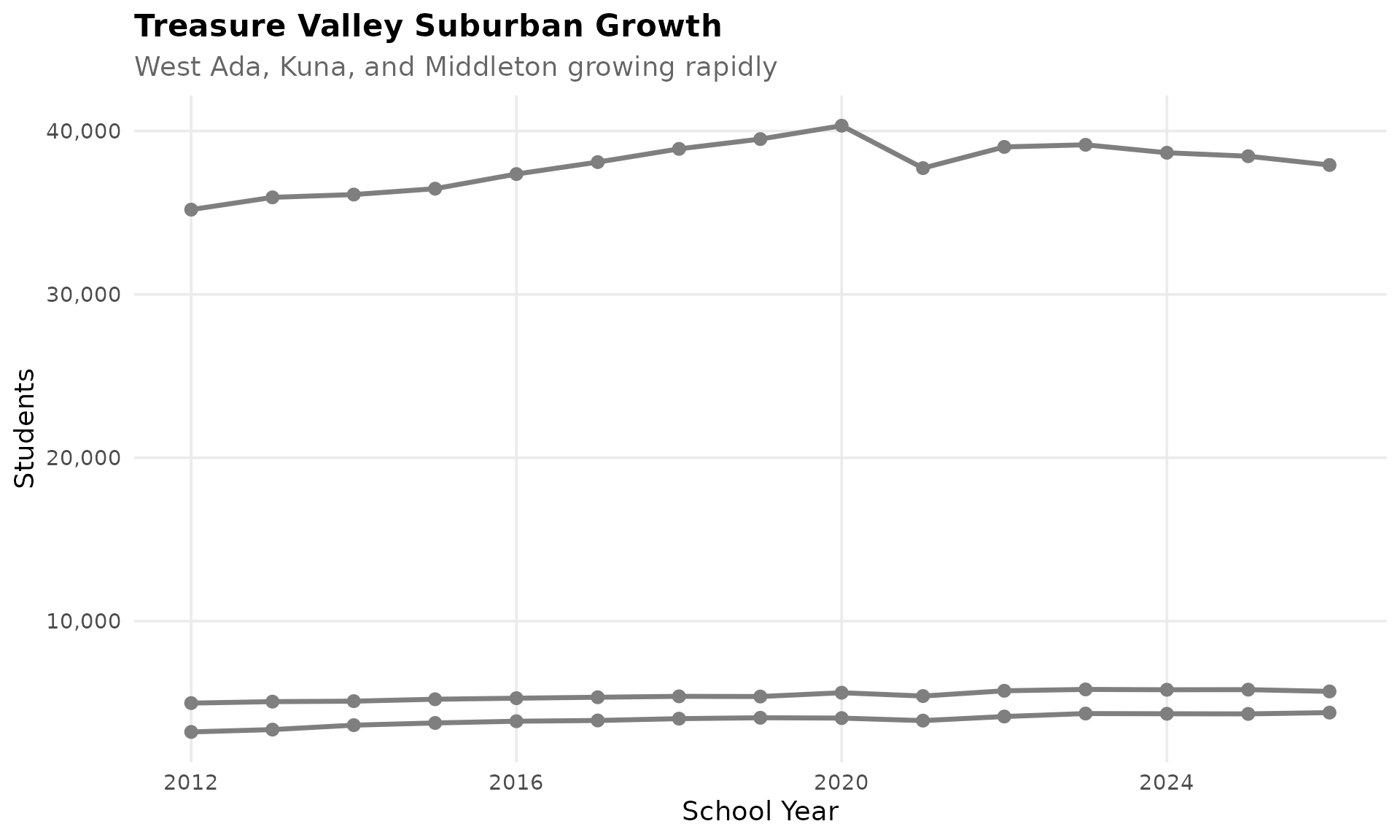
4. Kindergarten enrollment follows national trends
Like most states, Idaho’s kindergarten enrollment has declined in recent years as birth rates drop statewide. The decline appears to have stabilized since 2021.
k_trend <- enr_decade %>%
  filter(is_state, subgroup == "total_enrollment", grade_level == "K")
stopifnot(nrow(k_trend) > 0)
k_trend %>% select(end_year, n_students)
#>    end_year n_students
#> 1      2012      22044
#> 2      2013      22537
#> 3      2014      22506
#> 4      2015      21555
#> 5      2016      21115
#> 6      2017      21148
#> 7      2018      21170
#> 8      2019      21487
#> 9      2020      21940
#> 10     2021      21127
#> 11     2022      22060
#> 12     2023      22042
#> 13     2024      20658
#> 14     2025      20787
#> 15     2026      20184

ggplot(k_trend, aes(x = end_year, y = n_students)) +
  geom_line(linewidth = 1.5, color = colors["growth"]) +
  geom_point(size = 3, color = colors["growth"]) +
  scale_y_continuous(labels = comma) +
  labs(title = "Idaho Kindergarten Enrollment",
       subtitle = "Decline stabilized since 2021",
       x = "School Year", y = "Students") +
  theme_readme()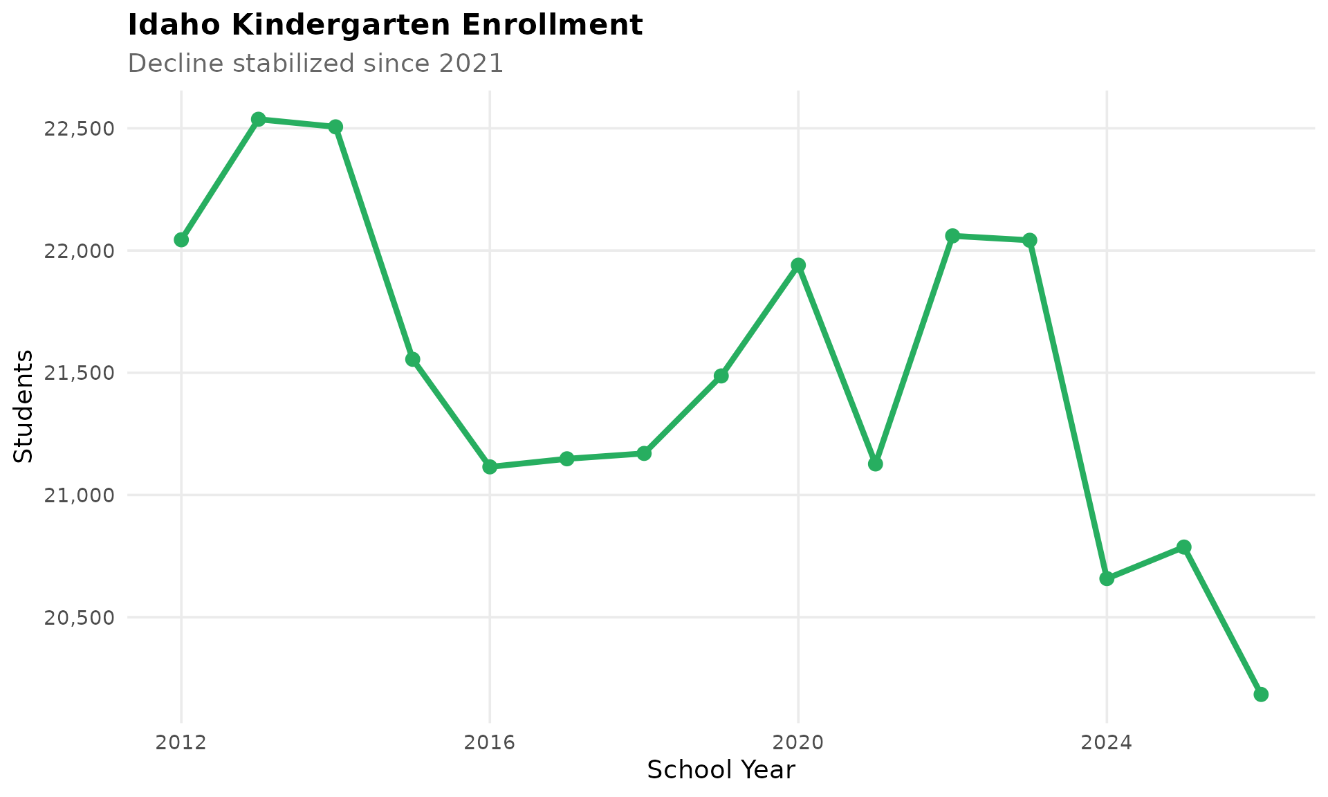
5. COVID barely slowed Idaho
Most states lost 3-5% enrollment during the pandemic. Idaho dipped briefly in 2020, then resumed growing. Families moved TO Idaho during the pandemic, offsetting any losses.
covid_years <- enr_all %>%
  filter(is_state, grade_level == "TOTAL", subgroup == "total_enrollment",
         end_year >= 2018)
stopifnot(nrow(covid_years) > 0)
covid_years %>% select(end_year, n_students)
#>   end_year n_students
#> 1     2018     302689
#> 2     2019     307228
#> 3     2020     311991
#> 4     2021     310653
#> 5     2022     316159
#> 6     2023     318979
#> 7     2024     318660
#> 8     2025     318067
#> 9     2026     314097

ggplot(covid_years, aes(x = end_year, y = n_students)) +
  geom_line(linewidth = 1.5, color = colors["total"]) +
  geom_point(size = 3, color = colors["total"]) +
  geom_vline(xintercept = 2021, linetype = "dashed", color = "red", alpha = 0.5) +
  annotate("text", x = 2021.3, y = max(covid_years$n_students, na.rm = TRUE) * 0.98,
           label = "COVID", hjust = 0, color = "red") +
  scale_y_continuous(labels = comma, limits = c(0, NA)) +
  labs(title = "Idaho Barely Slowed During COVID",
       subtitle = "Brief dip before resuming growth (2020-21 marked)",
       x = "School Year", y = "Students") +
  theme_readme()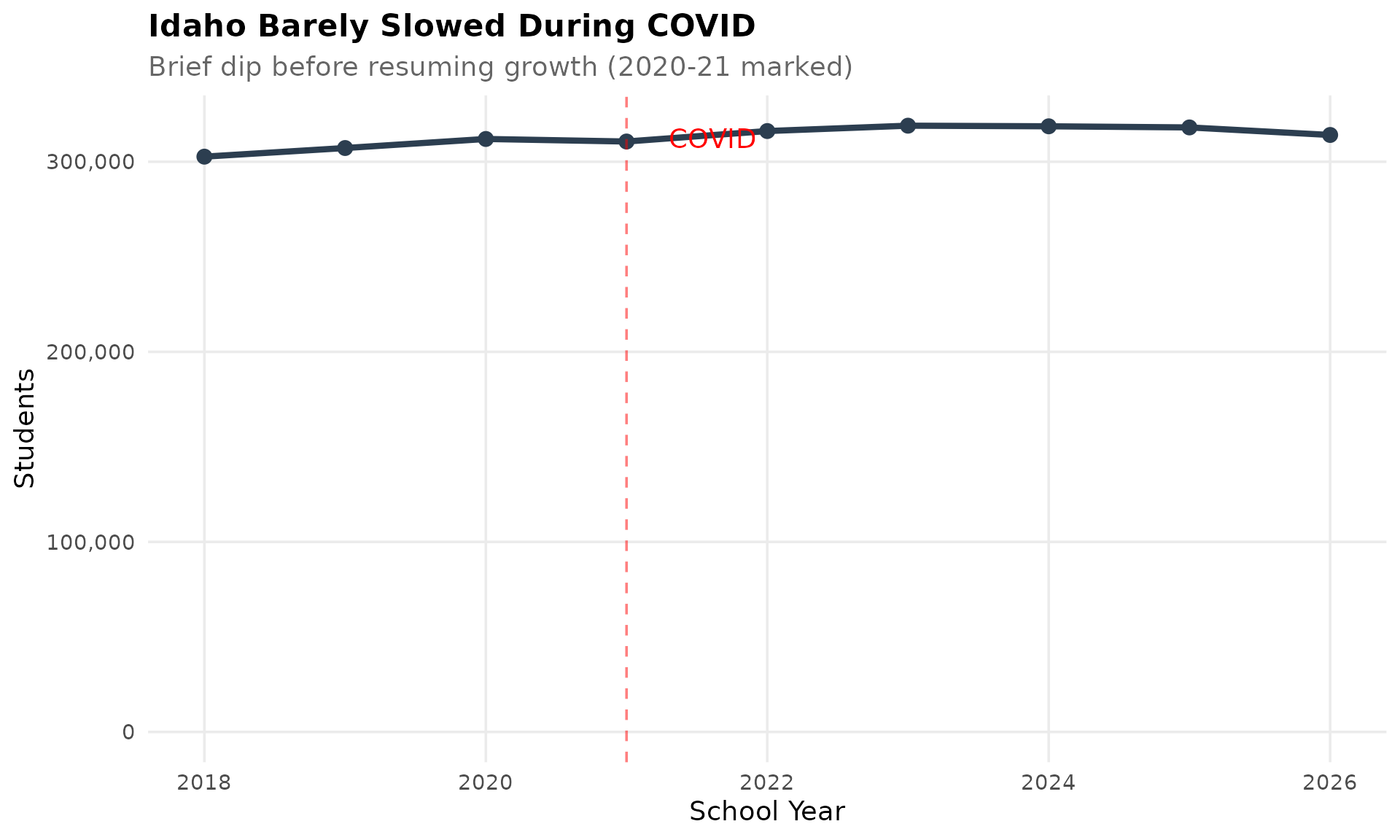
6. Charter schools serve 1 in 14 Idaho students
Idaho has 32 charter schools serving nearly 23,000 students. Idaho Home Learning Academy alone accounts for over 7,500 students - a third of all charter enrollment.
charter <- enr_current %>%
  filter(is_charter, grade_level == "TOTAL", subgroup == "total_enrollment")
stopifnot(nrow(charter) > 0)

charter_total <- sum(charter$n_students, na.rm = TRUE)
state_total <- enr_current %>%
  filter(is_state, grade_level == "TOTAL", subgroup == "total_enrollment") %>%
  pull(n_students)
charter_ratio <- round(state_total / charter_total)

charter %>%
  arrange(desc(n_students)) %>%
  head(10) %>%
  select(district_name, n_students)
#>                          district_name n_students
#> 1  IDAHO HOME LEARNING ACADEMY CHARTER       7504
#> 2          INSPIRE VIRTUAL CHARTER LEA       1553
#> 3                   IDAHO ARTS CHARTER       1421
#> 4         COMPAS PUBLIC CHARTER SCHOOL       1289
#> 5                   NORTH STAR CHARTER       1143
#> 6                VISION CHARTER SCHOOL        757
#> 7                XAVIER CHARTER SCHOOL        675
#> 8            WHITE PINE CHARTER SCHOOL        653
#> 9                 ANSER CHARTER SCHOOL        598
#> 10       COEUR D'ALENE CHARTER ACADEMY        593

charter %>%
  arrange(desc(n_students)) %>%
  head(10) %>%
  ggplot(aes(x = reorder(district_name, n_students), y = n_students)) +
  geom_col(fill = colors["district3"]) +
  coord_flip() +
  scale_y_continuous(labels = comma) +
  labs(title = "Idaho's Largest Charter Schools",
       subtitle = paste0(format(charter_total, big.mark = ","),
                        " students in charters (",
                        round(charter_total / state_total * 100, 1),
                        "% of state, 1 in ", charter_ratio, ")"),
       x = "", y = "Students") +
  theme_readme()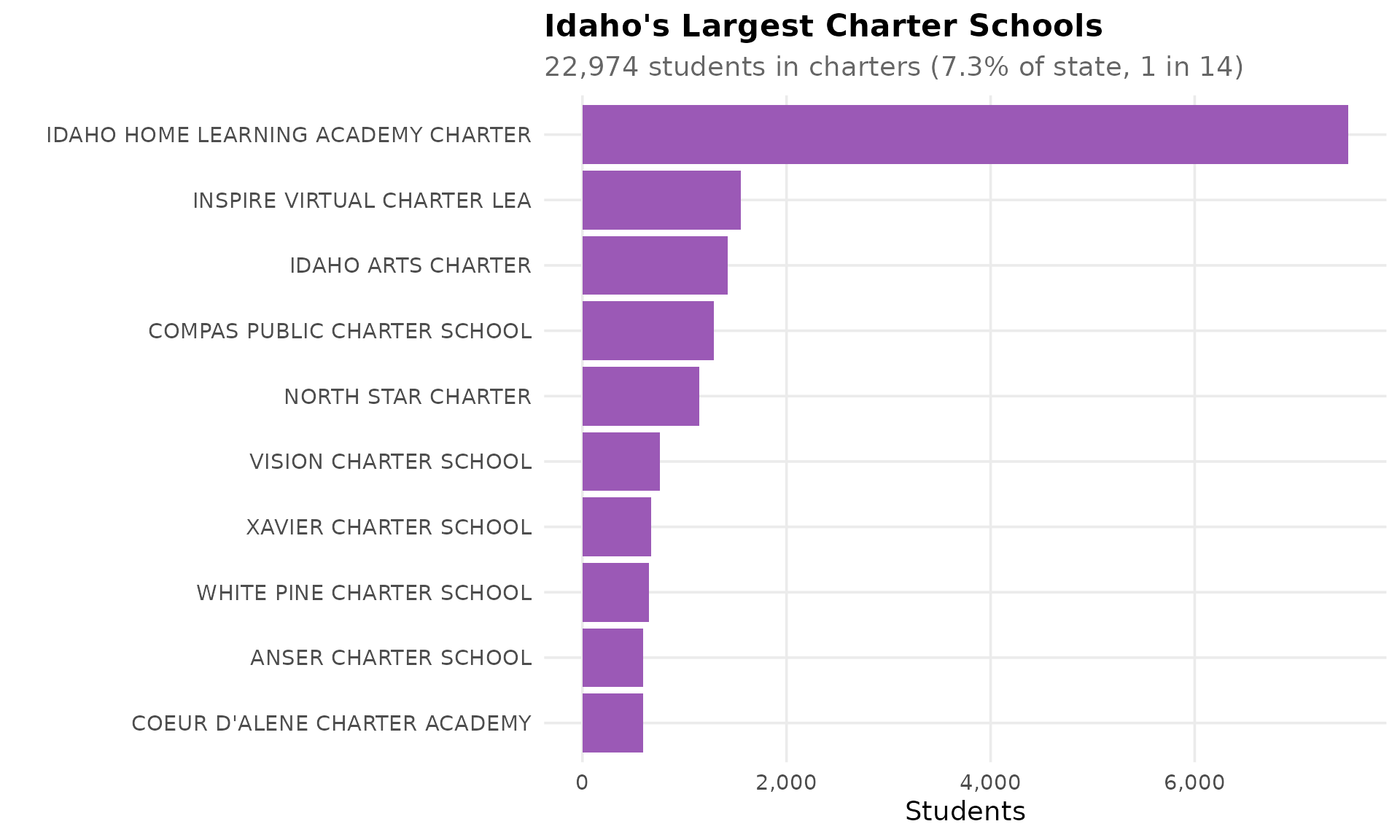
7. Rural Idaho is emptying out
While Boise suburbs boom, northern and eastern Idaho are hollowing out. Wallace (Silver Valley), Salmon, and Challis have lost half their students in 20 years.
rural <- c("WALLACE DISTRICT", "SALMON DISTRICT", "CHALLIS JOINT DISTRICT")
rural_trend <- enr_all %>%
  filter(is_district,
         grepl(paste(rural, collapse = "|"), district_name),
         subgroup == "total_enrollment", grade_level == "TOTAL")
stopifnot(nrow(rural_trend) > 0)
rural_trend %>% select(end_year, district_name, n_students)
#>    end_year          district_name n_students
#> 1      2002 CHALLIS JOINT DISTRICT        558
#> 2      2002        SALMON DISTRICT       1143
#> 3      2002       WALLACE DISTRICT        614
#> 4      2003 CHALLIS JOINT DISTRICT        520
#> 5      2003        SALMON DISTRICT       1112
#> 6      2003       WALLACE DISTRICT        599
#> 7      2004 CHALLIS JOINT DISTRICT        509
#> 8      2004        SALMON DISTRICT       1077
#> 9      2004       WALLACE DISTRICT        602
#> 10     2005 CHALLIS JOINT DISTRICT        461
#> 11     2005        SALMON DISTRICT       1060
#> 12     2005       WALLACE DISTRICT        555
#> 13     2006 CHALLIS JOINT DISTRICT        448
#> 14     2006        SALMON DISTRICT       1003
#> 15     2006       WALLACE DISTRICT        549
#> 16     2007 CHALLIS JOINT DISTRICT        462
#> 17     2007        SALMON DISTRICT        992
#> 18     2007       WALLACE DISTRICT        561
#> 19     2008 CHALLIS JOINT DISTRICT        467
#> 20     2008        SALMON DISTRICT        962
#> 21     2008       WALLACE DISTRICT        569
#> 22     2009 CHALLIS JOINT DISTRICT        439
#> 23     2009        SALMON DISTRICT        925
#> 24     2009       WALLACE DISTRICT        574
#> 25     2010 CHALLIS JOINT DISTRICT        411
#> 26     2010        SALMON DISTRICT        861
#> 27     2010       WALLACE DISTRICT        505
#> 28     2011 CHALLIS JOINT DISTRICT        430
#> 29     2011        SALMON DISTRICT        857
#> 30     2011       WALLACE DISTRICT        552
#> 31     2012 CHALLIS JOINT DISTRICT        439
#> 32     2012        SALMON DISTRICT        798
#> 33     2012       WALLACE DISTRICT        501
#> 34     2013 CHALLIS JOINT DISTRICT        433
#> 35     2013        SALMON DISTRICT        801
#> 36     2013       WALLACE DISTRICT        538
#> 37     2014 CHALLIS JOINT DISTRICT        408
#> 38     2014        SALMON DISTRICT        786
#> 39     2014       WALLACE DISTRICT        537
#> 40     2015 CHALLIS JOINT DISTRICT        403
#> 41     2015        SALMON DISTRICT        798
#> 42     2015       WALLACE DISTRICT        529
#> 43     2016 CHALLIS JOINT DISTRICT        376
#> 44     2016        SALMON DISTRICT        766
#> 45     2016       WALLACE DISTRICT        502
#> 46     2017 CHALLIS JOINT DISTRICT        360
#> 47     2017        SALMON DISTRICT        792
#> 48     2017       WALLACE DISTRICT        515
#> 49     2018 CHALLIS JOINT DISTRICT        354
#> 50     2018        SALMON DISTRICT        817
#> 51     2018       WALLACE DISTRICT        488
#> 52     2019 CHALLIS JOINT DISTRICT        362
#> 53     2019        SALMON DISTRICT        802
#> 54     2019       WALLACE DISTRICT        495
#> 55     2020 CHALLIS JOINT DISTRICT        324
#> 56     2020        SALMON DISTRICT        778
#> 57     2020       WALLACE DISTRICT        496
#> 58     2021 CHALLIS JOINT DISTRICT        307
#> 59     2021        SALMON DISTRICT        685
#> 60     2021       WALLACE DISTRICT        460
#> 61     2022 CHALLIS JOINT DISTRICT        345
#> 62     2022        SALMON DISTRICT        669
#> 63     2022       WALLACE DISTRICT        526
#> 64     2023 CHALLIS JOINT DISTRICT        333
#> 65     2023        SALMON DISTRICT        683
#> 66     2023       WALLACE DISTRICT        512
#> 67     2024 CHALLIS JOINT DISTRICT        345
#> 68     2024        SALMON DISTRICT        674
#> 69     2024       WALLACE DISTRICT        490
#> 70     2025 CHALLIS JOINT DISTRICT        343
#> 71     2025        SALMON DISTRICT        653
#> 72     2025       WALLACE DISTRICT        490
#> 73     2026 CHALLIS JOINT DISTRICT        329
#> 74     2026        SALMON DISTRICT        609
#> 75     2026       WALLACE DISTRICT        511

ggplot(rural_trend, aes(x = end_year, y = n_students, color = district_name)) +
  geom_line(linewidth = 1.2) +
  geom_point(size = 2) +
  scale_y_continuous(labels = comma) +
  scale_color_manual(values = c(colors["decline"], colors["district2"], colors["district3"])) +
  labs(title = "Rural Idaho is Emptying Out",
       subtitle = "Northern mountain communities losing students",
       x = "School Year", y = "Students", color = "") +
  theme_readme()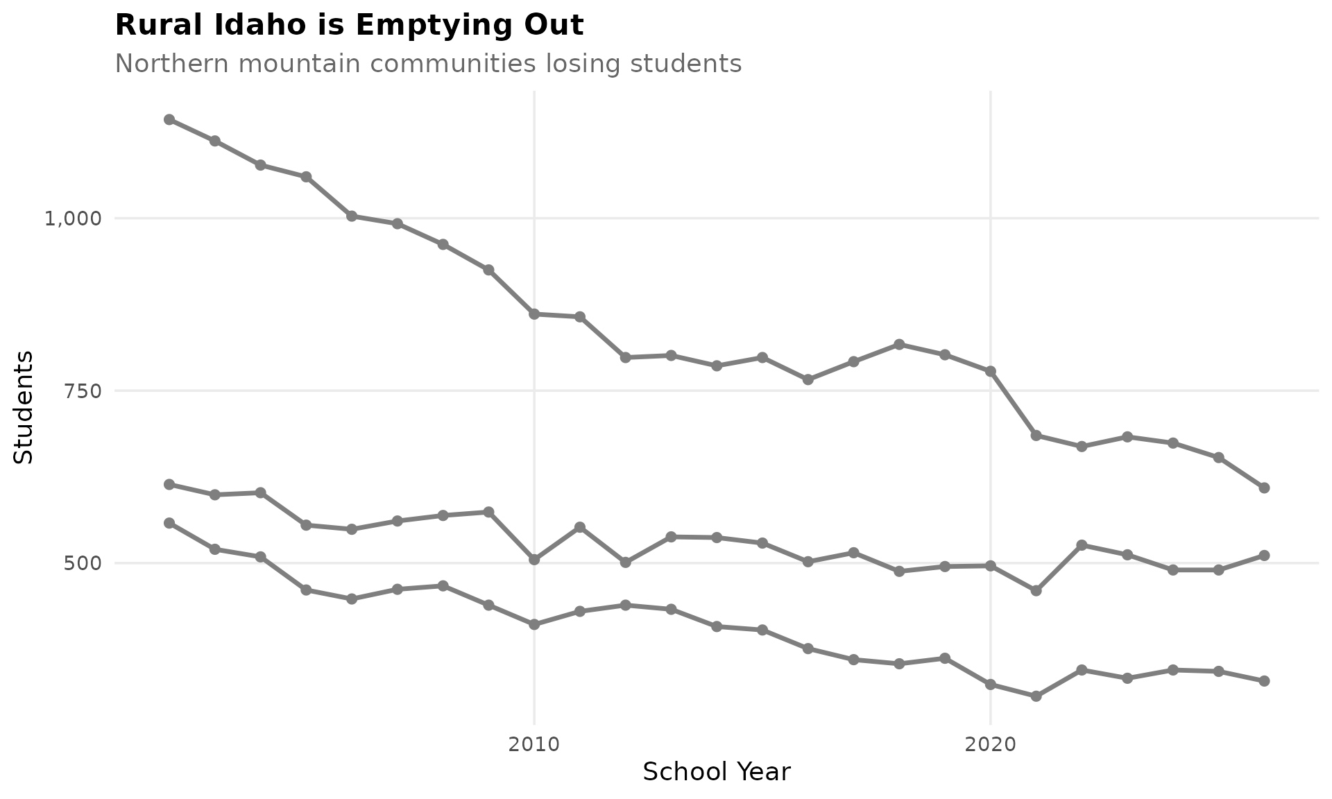
8. Boise proper declined while suburbs exploded
Boise Independent School District has declined to 22,000 students. Meanwhile, neighboring West Ada has grown from 20,000 to nearly 38,000. The growth is all in the suburbs.
boise_westada <- enr_all %>%
  filter(is_district,
         grepl("^BOISE INDEPENDENT DISTRICT|^WEST ADA DISTRICT", district_name),
         subgroup == "total_enrollment", grade_level == "TOTAL")
stopifnot(nrow(boise_westada) > 0)
boise_westada %>% select(end_year, district_name, n_students)
#>    end_year              district_name n_students
#> 1      2002 BOISE INDEPENDENT DISTRICT      26321
#> 2      2002          WEST ADA DISTRICT      25061
#> 3      2003 BOISE INDEPENDENT DISTRICT      25931
#> 4      2003          WEST ADA DISTRICT      25940
#> 5      2004 BOISE INDEPENDENT DISTRICT      25694
#> 6      2004          WEST ADA DISTRICT      26045
#> 7      2005 BOISE INDEPENDENT DISTRICT      25681
#> 8      2005          WEST ADA DISTRICT      28005
#> 9      2006 BOISE INDEPENDENT DISTRICT      25142
#> 10     2006          WEST ADA DISTRICT      30326
#> 11     2007 BOISE INDEPENDENT DISTRICT      24900
#> 12     2007          WEST ADA DISTRICT      31603
#> 13     2008 BOISE INDEPENDENT DISTRICT      24996
#> 14     2008          WEST ADA DISTRICT      32728
#> 15     2009 BOISE INDEPENDENT DISTRICT      24896
#> 16     2009          WEST ADA DISTRICT      33578
#> 17     2010 BOISE INDEPENDENT DISTRICT      25205
#> 18     2010          WEST ADA DISTRICT      34398
#> 19     2011 BOISE INDEPENDENT DISTRICT      25269
#> 20     2011          WEST ADA DISTRICT      34625
#> 21     2012 BOISE INDEPENDENT DISTRICT      25247
#> 22     2012          WEST ADA DISTRICT      35188
#> 23     2013 BOISE INDEPENDENT DISTRICT      25440
#> 24     2013          WEST ADA DISTRICT      35939
#> 25     2014 BOISE INDEPENDENT DISTRICT      25978
#> 26     2014          WEST ADA DISTRICT      36111
#> 27     2015 BOISE INDEPENDENT DISTRICT      25916
#> 28     2015          WEST ADA DISTRICT      36471
#> 29     2016 BOISE INDEPENDENT DISTRICT      25891
#> 30     2016          WEST ADA DISTRICT      37366
#> 31     2017 BOISE INDEPENDENT DISTRICT      26175
#> 32     2017          WEST ADA DISTRICT      38097
#> 33     2018 BOISE INDEPENDENT DISTRICT      26048
#> 34     2018          WEST ADA DISTRICT      38907
#> 35     2019 BOISE INDEPENDENT DISTRICT      25527
#> 36     2019          WEST ADA DISTRICT      39507
#> 37     2020 BOISE INDEPENDENT DISTRICT      25484
#> 38     2020          WEST ADA DISTRICT      40326
#> 39     2021 BOISE INDEPENDENT DISTRICT      23854
#> 40     2021          WEST ADA DISTRICT      37729
#> 41     2022 BOISE INDEPENDENT DISTRICT      23362
#> 42     2022          WEST ADA DISTRICT      39027
#> 43     2023 BOISE INDEPENDENT DISTRICT      22885
#> 44     2023          WEST ADA DISTRICT      39157
#> 45     2024 BOISE INDEPENDENT DISTRICT      22496
#> 46     2024          WEST ADA DISTRICT      38670
#> 47     2025 BOISE INDEPENDENT DISTRICT      22230
#> 48     2025          WEST ADA DISTRICT      38457
#> 49     2026 BOISE INDEPENDENT DISTRICT      21717
#> 50     2026          WEST ADA DISTRICT      37919

ggplot(boise_westada, aes(x = end_year, y = n_students, color = district_name)) +
  geom_line(linewidth = 1.2) +
  geom_point(size = 2.5) +
  scale_y_continuous(labels = comma) +
  scale_color_manual(values = c(colors["district1"], colors["district2"])) +
  labs(title = "Boise Flat, West Ada Exploding",
       subtitle = "Suburban growth outpacing the urban core",
       x = "School Year", y = "Students", color = "") +
  theme_readme()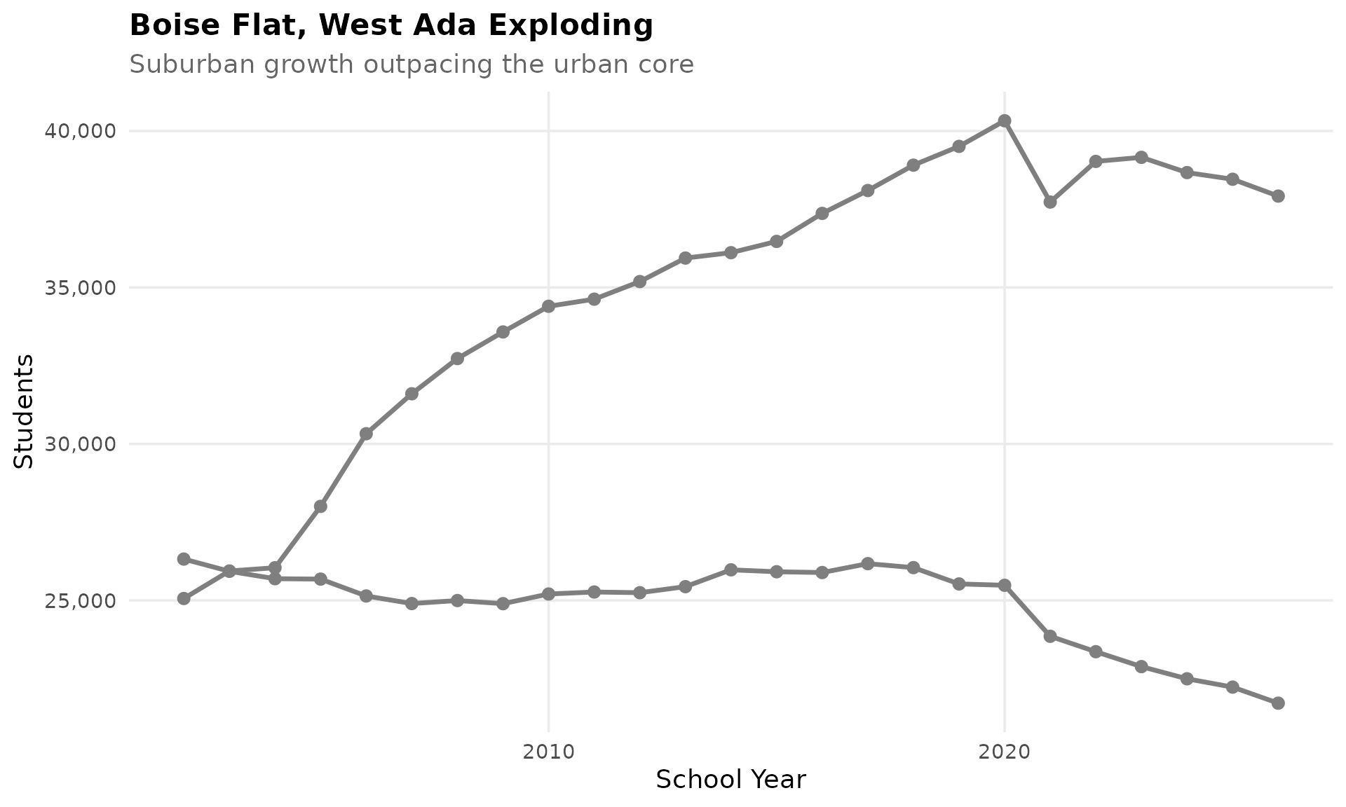
9. High school enrollment surged 22% in 15 years
Idaho’s high schools are seeing record enrollment as the wave of growth works through the grades.
hs_trend <- enr_decade %>%
  filter(is_state, subgroup == "total_enrollment",
         grade_level %in% c("09", "10", "11", "12")) %>%
  group_by(end_year) %>%
  summarize(n_students = sum(n_students, na.rm = TRUE), .groups = "drop")
stopifnot(nrow(hs_trend) > 0)

# Compute growth dynamically
hs_first <- hs_trend$n_students[1]
hs_last <- hs_trend$n_students[nrow(hs_trend)]
hs_pct <- round((hs_last / hs_first - 1) * 100)

hs_trend
#> # A tibble: 15 × 2
#>    end_year n_students
#>       <int>      <dbl>
#>  1     2012     83121
#>  2     2013     83856
#>  3     2014     84548.
#>  4     2015     85212
#>  5     2016     87524
#>  6     2017     89206
#>  7     2018     90845
#>  8     2019     92165
#>  9     2020     94603
#> 10     2021     97596
#> 11     2022     98764
#> 12     2023    100362
#> 13     2024    101530
#> 14     2025    102039
#> 15     2026    101402
cat("HS growth:", format(hs_first, big.mark = ","), "->",
    format(hs_last, big.mark = ","), "(+", hs_pct, "%)\n")
#> HS growth: 83,121 -> 101,402 (+ 22 %)

ggplot(hs_trend, aes(x = end_year, y = n_students)) +
  geom_line(linewidth = 1.5, color = colors["total"]) +
  geom_point(size = 3, color = colors["total"]) +
  scale_y_continuous(labels = comma, limits = c(0, NA)) +
  labs(title = "Idaho High School Enrollment (Grades 9-12)",
       subtitle = paste0("From ", format(hs_first, big.mark = ","), " to ",
                        format(hs_last, big.mark = ","), " (+", hs_pct, "%)"),
       x = "School Year", y = "Students") +
  theme_readme()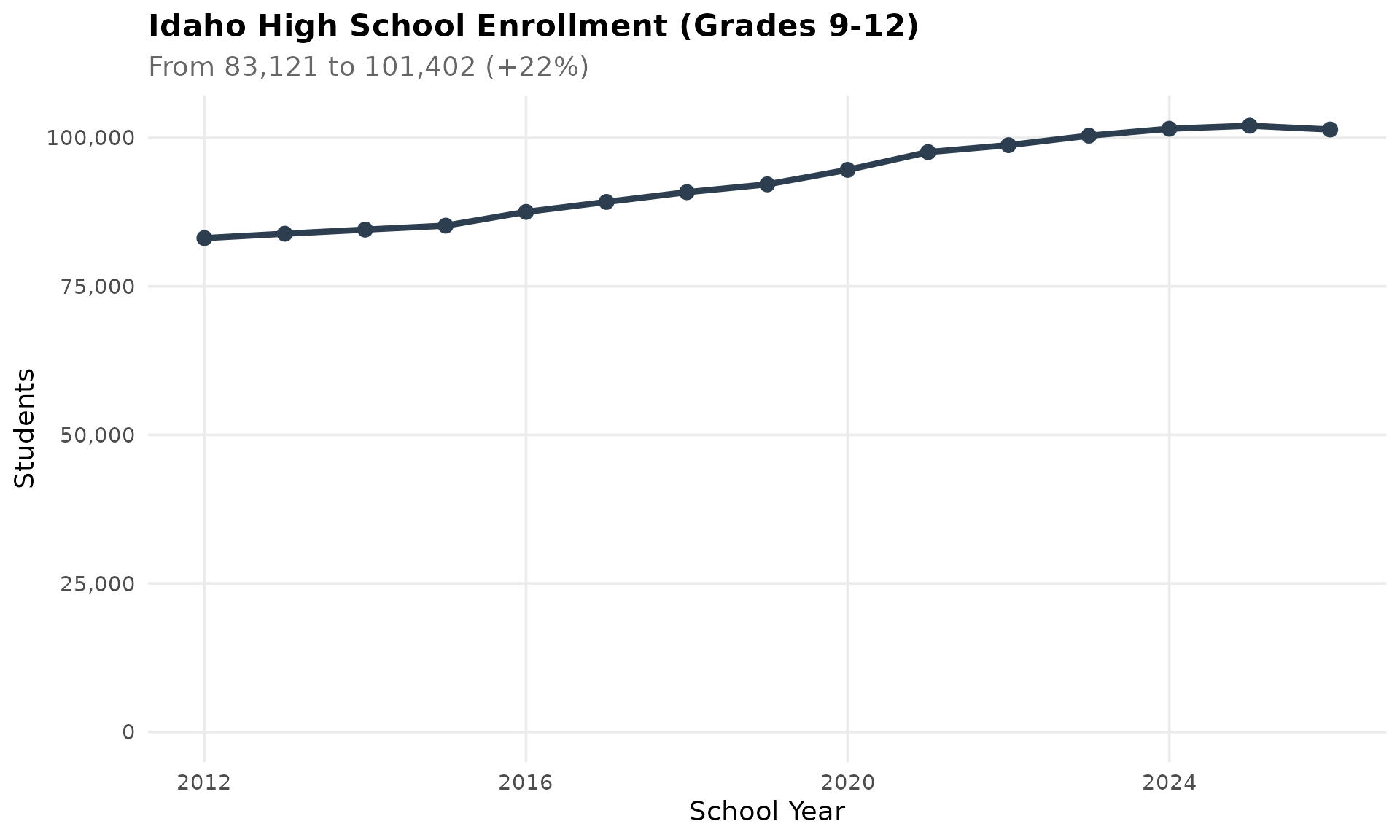
10. The Magic Valley is holding steady
Twin Falls, Jerome, and Minidoka County in south-central Idaho have maintained steady enrollment even as some rural areas shrink. Agriculture and food processing anchor these communities.
magic_valley <- c("TWIN FALLS DISTRICT", "JEROME JOINT DISTRICT", "MINIDOKA COUNTY JOINT DISTRICT")
mv_trend <- enr_decade %>%
  filter(is_district,
         grepl(paste(magic_valley, collapse = "|"), district_name),
         !grepl("VIRTUAL|CHARTER", district_name),
         subgroup == "total_enrollment", grade_level == "TOTAL")
stopifnot(nrow(mv_trend) > 0)
mv_trend %>% select(end_year, district_name, n_students)
#>    end_year                  district_name n_students
#> 1      2012          JEROME JOINT DISTRICT       3428
#> 2      2012 MINIDOKA COUNTY JOINT DISTRICT       4042
#> 3      2012            TWIN FALLS DISTRICT       7791
#> 4      2013          JEROME JOINT DISTRICT       3590
#> 5      2013 MINIDOKA COUNTY JOINT DISTRICT       4016
#> 6      2013            TWIN FALLS DISTRICT       8265
#> 7      2014          JEROME JOINT DISTRICT       3645
#> 8      2014 MINIDOKA COUNTY JOINT DISTRICT       4098
#> 9      2014            TWIN FALLS DISTRICT       8565
#> 10     2015          JEROME JOINT DISTRICT       3752
#> 11     2015 MINIDOKA COUNTY JOINT DISTRICT       4127
#> 12     2015            TWIN FALLS DISTRICT       8805
#> 13     2016          JEROME JOINT DISTRICT       3830
#> 14     2016 MINIDOKA COUNTY JOINT DISTRICT       4180
#> 15     2016            TWIN FALLS DISTRICT       9051
#> 16     2017          JEROME JOINT DISTRICT       3933
#> 17     2017 MINIDOKA COUNTY JOINT DISTRICT       4232
#> 18     2017            TWIN FALLS DISTRICT       9194
#> 19     2018          JEROME JOINT DISTRICT       4014
#> 20     2018 MINIDOKA COUNTY JOINT DISTRICT       4222
#> 21     2018            TWIN FALLS DISTRICT       9478
#> 22     2019          JEROME JOINT DISTRICT       4062
#> 23     2019 MINIDOKA COUNTY JOINT DISTRICT       4257
#> 24     2019            TWIN FALLS DISTRICT       9488
#> 25     2020          JEROME JOINT DISTRICT       4141
#> 26     2020 MINIDOKA COUNTY JOINT DISTRICT       4315
#> 27     2020            TWIN FALLS DISTRICT       9620
#> 28     2021          JEROME JOINT DISTRICT       4076
#> 29     2021 MINIDOKA COUNTY JOINT DISTRICT       4264
#> 30     2021            TWIN FALLS DISTRICT       9180
#> 31     2022          JEROME JOINT DISTRICT       4151
#> 32     2022 MINIDOKA COUNTY JOINT DISTRICT       4480
#> 33     2022            TWIN FALLS DISTRICT       9412
#> 34     2023          JEROME JOINT DISTRICT       4155
#> 35     2023 MINIDOKA COUNTY JOINT DISTRICT       4420
#> 36     2023            TWIN FALLS DISTRICT       9362
#> 37     2024          JEROME JOINT DISTRICT       4082
#> 38     2024 MINIDOKA COUNTY JOINT DISTRICT       4414
#> 39     2024            TWIN FALLS DISTRICT       9241
#> 40     2025          JEROME JOINT DISTRICT       4006
#> 41     2025 MINIDOKA COUNTY JOINT DISTRICT       4293
#> 42     2025            TWIN FALLS DISTRICT       9024
#> 43     2026          JEROME JOINT DISTRICT       3862
#> 44     2026 MINIDOKA COUNTY JOINT DISTRICT       4114
#> 45     2026            TWIN FALLS DISTRICT       8774

ggplot(mv_trend, aes(x = end_year, y = n_students, color = district_name)) +
  geom_line(linewidth = 1.2) +
  geom_point(size = 2.5) +
  scale_y_continuous(labels = comma) +
  scale_color_manual(values = c(colors["district1"], colors["district2"], colors["district3"])) +
  labs(title = "Magic Valley Districts Holding Steady",
       subtitle = "Twin Falls and Jerome maintain enrollment",
       x = "School Year", y = "Students", color = "") +
  theme_readme()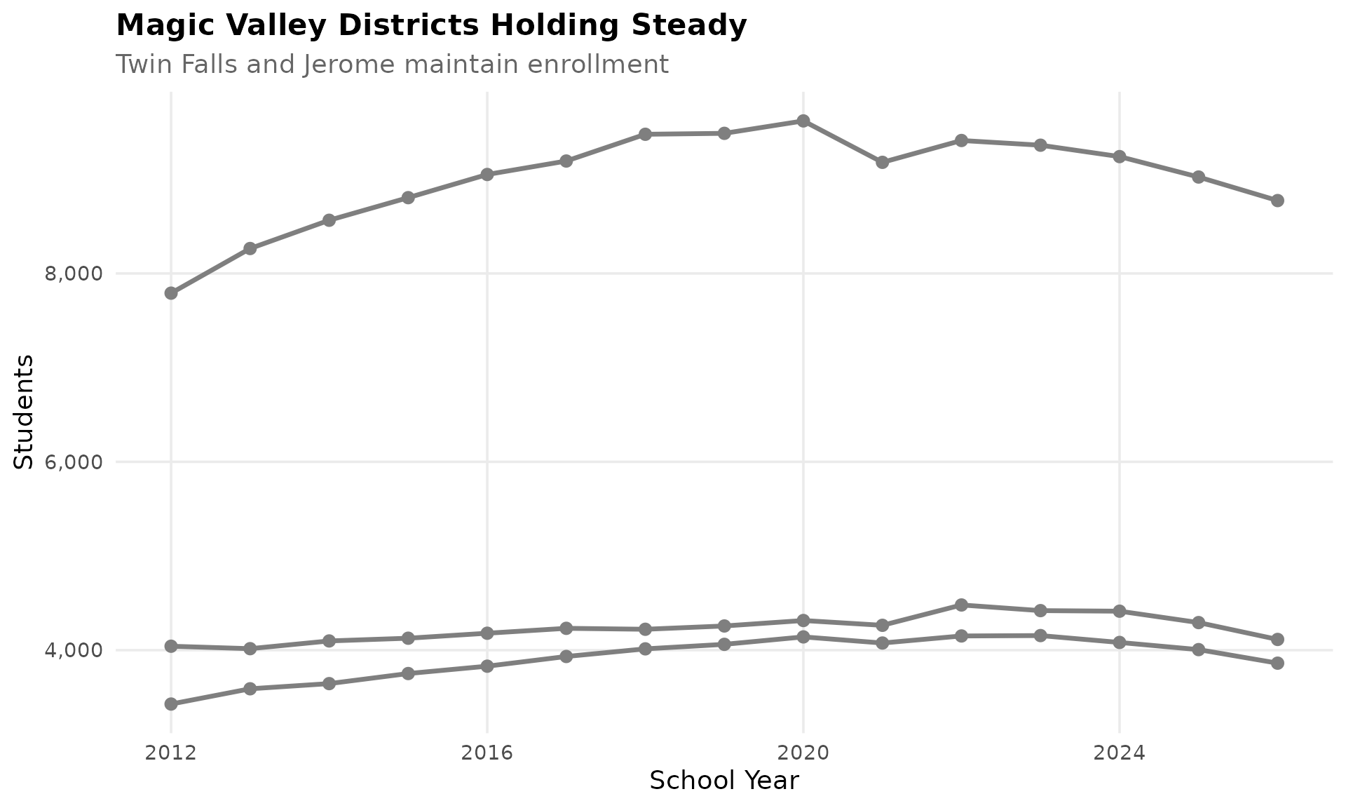
11. Elementary is the biggest cohort
Idaho’s elementary schools (K-5) serve the largest share of students. The grade distribution shows a healthy pipeline with growing younger grades - a sign of continued future growth.
grades <- enr_current %>%
  filter(is_state, subgroup == "total_enrollment",
         grade_level %in% c("K", "01", "02", "03", "04", "05",
                           "06", "07", "08", "09", "10", "11", "12"))
stopifnot(nrow(grades) > 0)

grade_order <- c("K", "01", "02", "03", "04", "05",
                 "06", "07", "08", "09", "10", "11", "12")
grades$grade_level <- factor(grades$grade_level, levels = grade_order)

grades %>% select(grade_level, n_students)
#>    grade_level n_students
#> 1            K      20184
#> 2           01      21286
#> 3           02      21524
#> 4           03      23354
#> 5           04      24147
#> 6           05      24290
#> 7           06      24539
#> 8           07      24756
#> 9           08      24762
#> 10          09      25474
#> 11          10      25413
#> 12          11      25199
#> 13          12      25316

ggplot(grades, aes(x = grade_level, y = n_students)) +
  geom_col(fill = colors["total"]) +
  scale_y_continuous(labels = comma) +
  labs(title = "Idaho Enrollment by Grade Level",
       subtitle = "Strong elementary enrollment signals continued growth",
       x = "Grade", y = "Students") +
  theme_readme()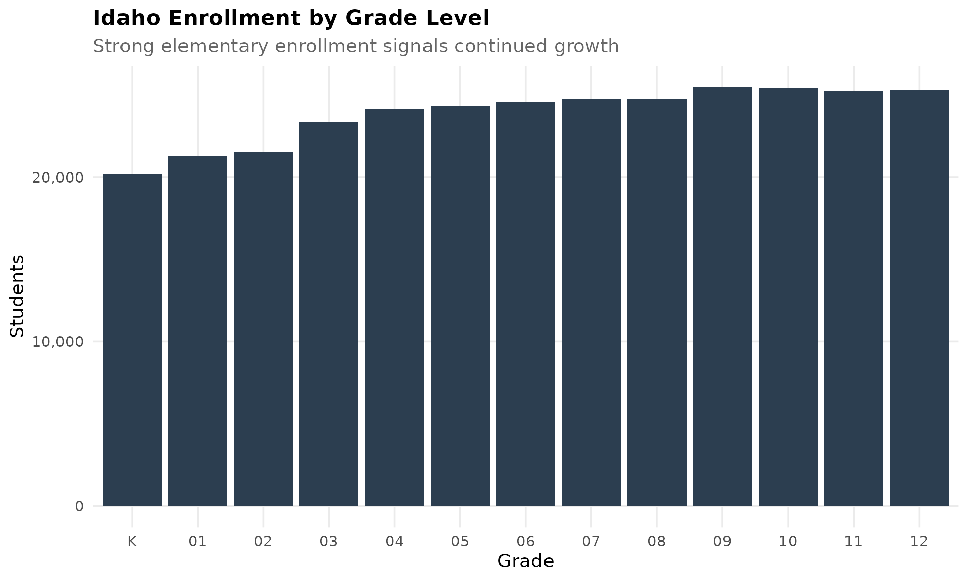
12. Coeur d’Alene leads northern Idaho
In the Idaho panhandle, Coeur d’Alene School District leads with nearly 10,000 students. Post Falls and Lakeland are also growing as people relocate from Spokane and beyond.
north <- c("COEUR D ALENE DISTRICT", "POST FALLS DISTRICT", "LAKELAND DISTRICT")
north_trend <- enr_decade %>%
  filter(is_district,
         grepl(paste(north, collapse = "|"), district_name),
         subgroup == "total_enrollment", grade_level == "TOTAL")
stopifnot(nrow(north_trend) > 0)
north_trend %>% select(end_year, district_name, n_students)
#>    end_year          district_name n_students
#> 1      2012 COEUR D ALENE DISTRICT      10107
#> 2      2012      LAKELAND DISTRICT       4340
#> 3      2012    POST FALLS DISTRICT       5626
#> 4      2013 COEUR D ALENE DISTRICT      10173
#> 5      2013      LAKELAND DISTRICT       4164
#> 6      2013    POST FALLS DISTRICT       5697
#> 7      2014 COEUR D ALENE DISTRICT      10284
#> 8      2014      LAKELAND DISTRICT       4130
#> 9      2014    POST FALLS DISTRICT       5706
#> 10     2015 COEUR D ALENE DISTRICT      10458
#> 11     2015      LAKELAND DISTRICT       4199
#> 12     2015    POST FALLS DISTRICT       5629
#> 13     2016 COEUR D ALENE DISTRICT      10711
#> 14     2016      LAKELAND DISTRICT       4215
#> 15     2016    POST FALLS DISTRICT       5718
#> 16     2017 COEUR D ALENE DISTRICT      10700
#> 17     2017      LAKELAND DISTRICT       4381
#> 18     2017    POST FALLS DISTRICT       5809
#> 19     2018 COEUR D ALENE DISTRICT      10836
#> 20     2018      LAKELAND DISTRICT       4371
#> 21     2018    POST FALLS DISTRICT       5897
#> 22     2019 COEUR D ALENE DISTRICT      10888
#> 23     2019      LAKELAND DISTRICT       4474
#> 24     2019    POST FALLS DISTRICT       6055
#> 25     2020 COEUR D ALENE DISTRICT      11075
#> 26     2020      LAKELAND DISTRICT       4590
#> 27     2020    POST FALLS DISTRICT       6175
#> 28     2021 COEUR D ALENE DISTRICT      10061
#> 29     2021      LAKELAND DISTRICT       4320
#> 30     2021    POST FALLS DISTRICT       5842
#> 31     2022 COEUR D ALENE DISTRICT      10191
#> 32     2022      LAKELAND DISTRICT       4671
#> 33     2022    POST FALLS DISTRICT       6194
#> 34     2023 COEUR D ALENE DISTRICT      10137
#> 35     2023      LAKELAND DISTRICT       4768
#> 36     2023    POST FALLS DISTRICT       6069
#> 37     2024 COEUR D ALENE DISTRICT       9677
#> 38     2024      LAKELAND DISTRICT       4602
#> 39     2024    POST FALLS DISTRICT       5911
#> 40     2025 COEUR D ALENE DISTRICT       9667
#> 41     2025      LAKELAND DISTRICT       4647
#> 42     2025    POST FALLS DISTRICT       5823
#> 43     2026 COEUR D ALENE DISTRICT       9680
#> 44     2026      LAKELAND DISTRICT       4649
#> 45     2026    POST FALLS DISTRICT       5838

ggplot(north_trend, aes(x = end_year, y = n_students, color = district_name)) +
  geom_line(linewidth = 1.2) +
  geom_point(size = 2.5) +
  scale_y_continuous(labels = comma) +
  scale_color_manual(values = c(colors["district1"], colors["district2"], colors["district3"])) +
  labs(title = "North Idaho District Growth",
       subtitle = "Coeur d'Alene, Post Falls, and Lakeland expanding",
       x = "School Year", y = "Students", color = "") +
  theme_readme()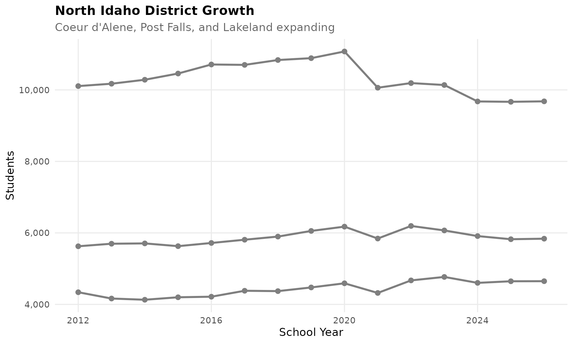
13. Small districts dominate the landscape
Idaho has 115+ school districts, but many are tiny. Over 40 districts have fewer than 500 students. These small rural districts face unique challenges with limited resources.
district_sizes <- enr_current %>%
  filter(is_district, grade_level == "TOTAL", subgroup == "total_enrollment") %>%
  mutate(size_category = case_when(
    n_students >= 10000 ~ "10,000+",
    n_students >= 5000 ~ "5,000-9,999",
    n_students >= 2000 ~ "2,000-4,999",
    n_students >= 1000 ~ "1,000-1,999",
    n_students >= 500 ~ "500-999",
    TRUE ~ "Under 500"
  )) %>%
  group_by(size_category) %>%
  summarize(n_districts = n(), .groups = "drop")
stopifnot(nrow(district_sizes) > 0)

district_sizes$size_category <- factor(district_sizes$size_category,
  levels = c("Under 500", "500-999", "1,000-1,999", "2,000-4,999", "5,000-9,999", "10,000+"))

district_sizes
#> # A tibble: 6 × 2
#>   size_category n_districts
#>   <fct>               <int>
#> 1 1,000-1,999            23
#> 2 10,000+                 6
#> 3 2,000-4,999            19
#> 4 5,000-9,999             9
#> 5 500-999                37
#> 6 Under 500              98

ggplot(district_sizes, aes(x = size_category, y = n_districts)) +
  geom_col(fill = colors["total"]) +
  labs(title = "Idaho Districts by Size",
       subtitle = "Many small rural districts, few large ones",
       x = "District Size (Students)", y = "Number of Districts") +
  theme_readme()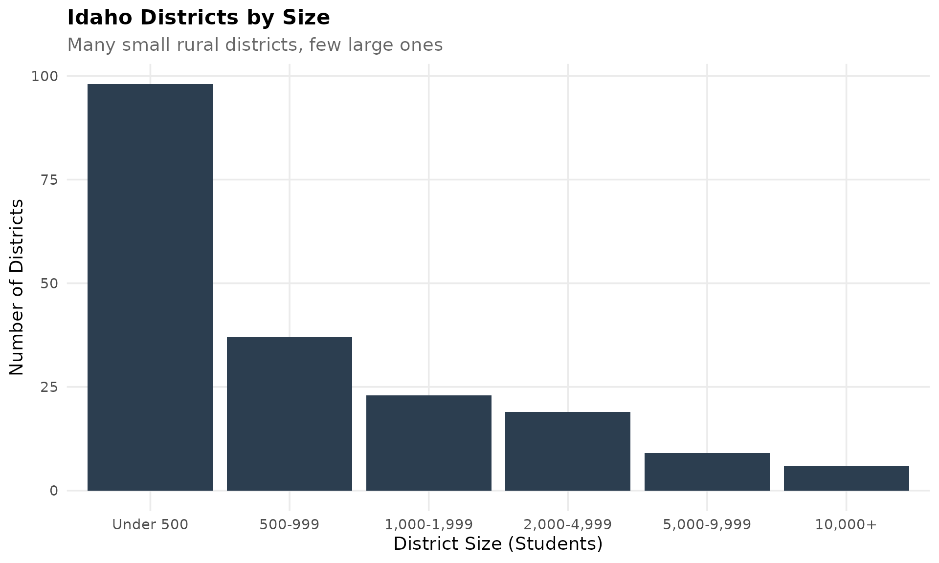
14. Nampa and Caldwell anchor Canyon County
Nampa School District and Caldwell serve Canyon County west of Boise. Both have grown with the Treasure Valley, though Nampa has seen recent declines from its 2014 peak.
canyon <- c("NAMPA SCHOOL DISTRICT", "CALDWELL DISTRICT")
canyon_trend <- enr_decade %>%
  filter(is_district,
         grepl(paste(canyon, collapse = "|"), district_name),
         subgroup == "total_enrollment", grade_level == "TOTAL")
stopifnot(nrow(canyon_trend) > 0)
canyon_trend %>% select(end_year, district_name, n_students)
#>    end_year         district_name n_students
#> 1      2012 NAMPA SCHOOL DISTRICT      15135
#> 2      2012     CALDWELL DISTRICT       5961
#> 3      2013 NAMPA SCHOOL DISTRICT      15776
#> 4      2013     CALDWELL DISTRICT       6151
#> 5      2014 NAMPA SCHOOL DISTRICT      15044
#> 6      2014     CALDWELL DISTRICT       6277
#> 7      2015 NAMPA SCHOOL DISTRICT      14901
#> 8      2015     CALDWELL DISTRICT       6173
#> 9      2016 NAMPA SCHOOL DISTRICT      14848
#> 10     2016     CALDWELL DISTRICT       6300
#> 11     2017 NAMPA SCHOOL DISTRICT      14341
#> 12     2017     CALDWELL DISTRICT       6338
#> 13     2018 NAMPA SCHOOL DISTRICT      14470
#> 14     2018     CALDWELL DISTRICT       6424
#> 15     2019 NAMPA SCHOOL DISTRICT      13977
#> 16     2019     CALDWELL DISTRICT       6407
#> 17     2020 NAMPA SCHOOL DISTRICT      14039
#> 18     2020     CALDWELL DISTRICT       6125
#> 19     2021 NAMPA SCHOOL DISTRICT      13230
#> 20     2021     CALDWELL DISTRICT       5595
#> 21     2022 NAMPA SCHOOL DISTRICT      13657
#> 22     2022     CALDWELL DISTRICT       5596
#> 23     2023 NAMPA SCHOOL DISTRICT      13418
#> 24     2023     CALDWELL DISTRICT       5508
#> 25     2024 NAMPA SCHOOL DISTRICT      13150
#> 26     2024     CALDWELL DISTRICT       5401
#> 27     2025 NAMPA SCHOOL DISTRICT      12729
#> 28     2025     CALDWELL DISTRICT       5142
#> 29     2026 NAMPA SCHOOL DISTRICT      12473
#> 30     2026     CALDWELL DISTRICT       4932

ggplot(canyon_trend, aes(x = end_year, y = n_students, color = district_name)) +
  geom_line(linewidth = 1.2) +
  geom_point(size = 2.5) +
  scale_y_continuous(labels = comma) +
  scale_color_manual(values = c(colors["district1"], colors["district2"])) +
  labs(title = "Canyon County Districts",
       subtitle = "Nampa and Caldwell growing with Treasure Valley",
       x = "School Year", y = "Students", color = "") +
  theme_readme()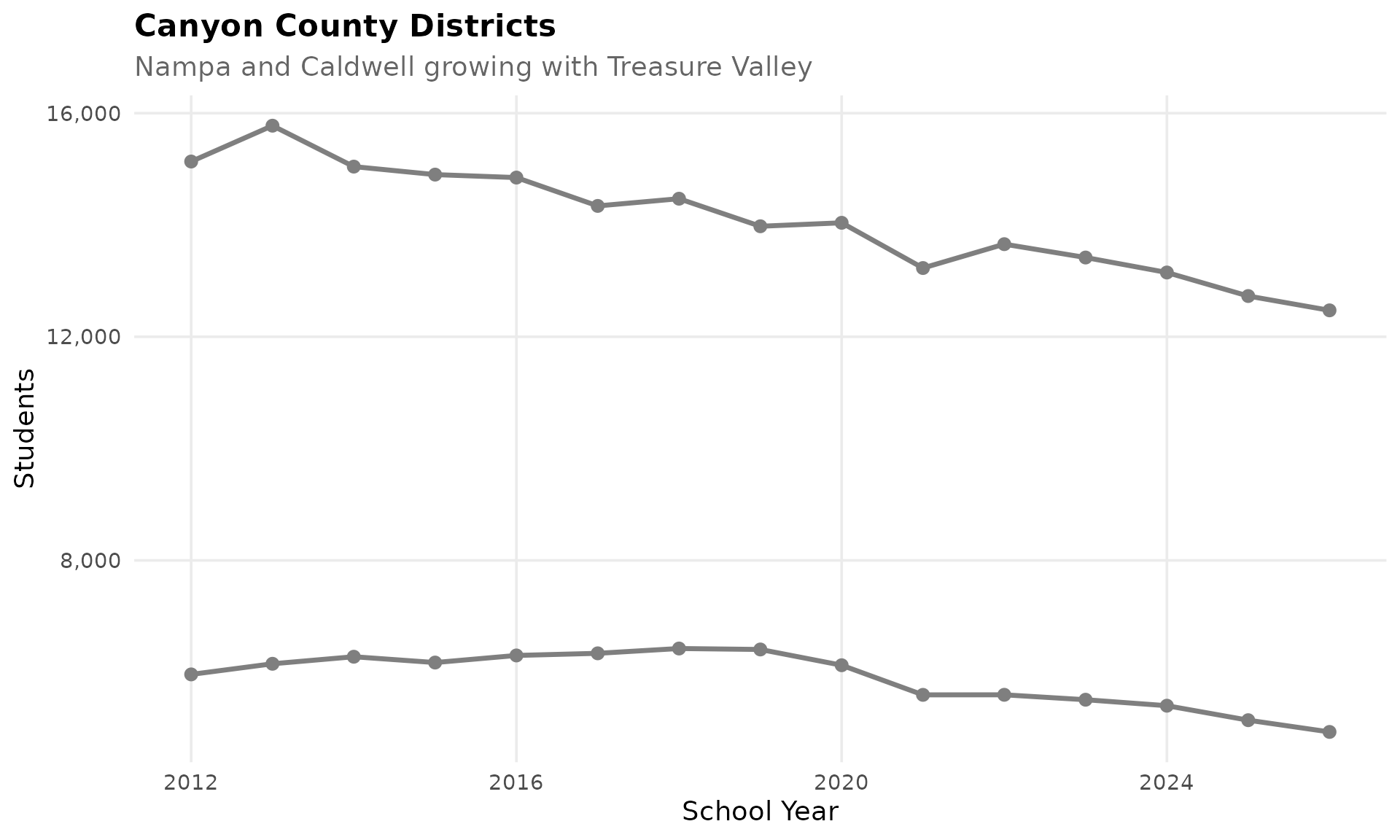
15. Idaho Falls leads eastern Idaho
Idaho Falls School District (#91) anchors the eastern region with nearly 10,000 students. Nearby Bonneville Joint District serves the growing suburban areas with 13,500 students. Eastern Idaho grows more slowly than the Treasure Valley.
eastern <- c("IDAHO FALLS DISTRICT", "BONNEVILLE JOINT DISTRICT")
eastern_trend <- enr_decade %>%
  filter(is_district,
         grepl(paste(eastern, collapse = "|"), district_name),
         subgroup == "total_enrollment", grade_level == "TOTAL")
stopifnot(nrow(eastern_trend) > 0)
eastern_trend %>% select(end_year, district_name, n_students)
#>    end_year             district_name n_students
#> 1      2012      IDAHO FALLS DISTRICT      10197
#> 2      2012 BONNEVILLE JOINT DISTRICT      10359
#> 3      2013      IDAHO FALLS DISTRICT      10499
#> 4      2013 BONNEVILLE JOINT DISTRICT      10834
#> 5      2014      IDAHO FALLS DISTRICT      10263
#> 6      2014 BONNEVILLE JOINT DISTRICT      11149
#> 7      2015      IDAHO FALLS DISTRICT      10391
#> 8      2015 BONNEVILLE JOINT DISTRICT      11870
#> 9      2016      IDAHO FALLS DISTRICT      10410
#> 10     2016 BONNEVILLE JOINT DISTRICT      11888
#> 11     2017      IDAHO FALLS DISTRICT      10257
#> 12     2017 BONNEVILLE JOINT DISTRICT      12224
#> 13     2018      IDAHO FALLS DISTRICT      10167
#> 14     2018 BONNEVILLE JOINT DISTRICT      12527
#> 15     2019      IDAHO FALLS DISTRICT      10213
#> 16     2019 BONNEVILLE JOINT DISTRICT      12905
#> 17     2020      IDAHO FALLS DISTRICT      10272
#> 18     2020 BONNEVILLE JOINT DISTRICT      13325
#> 19     2021      IDAHO FALLS DISTRICT      10005
#> 20     2021 BONNEVILLE JOINT DISTRICT      13224
#> 21     2022      IDAHO FALLS DISTRICT      10194
#> 22     2022 BONNEVILLE JOINT DISTRICT      13481
#> 23     2023      IDAHO FALLS DISTRICT      10255
#> 24     2023 BONNEVILLE JOINT DISTRICT      13801
#> 25     2024      IDAHO FALLS DISTRICT      10289
#> 26     2024 BONNEVILLE JOINT DISTRICT      13663
#> 27     2025      IDAHO FALLS DISTRICT       9935
#> 28     2025 BONNEVILLE JOINT DISTRICT      13604
#> 29     2026      IDAHO FALLS DISTRICT       9751
#> 30     2026 BONNEVILLE JOINT DISTRICT      13511

ggplot(eastern_trend, aes(x = end_year, y = n_students, color = district_name)) +
  geom_line(linewidth = 1.2) +
  geom_point(size = 2.5) +
  scale_y_continuous(labels = comma) +
  scale_color_manual(values = c(colors["district1"], colors["district2"])) +
  labs(title = "Eastern Idaho Districts",
       subtitle = "Idaho Falls and Bonneville anchor the region",
       x = "School Year", y = "Students", color = "") +
  theme_readme()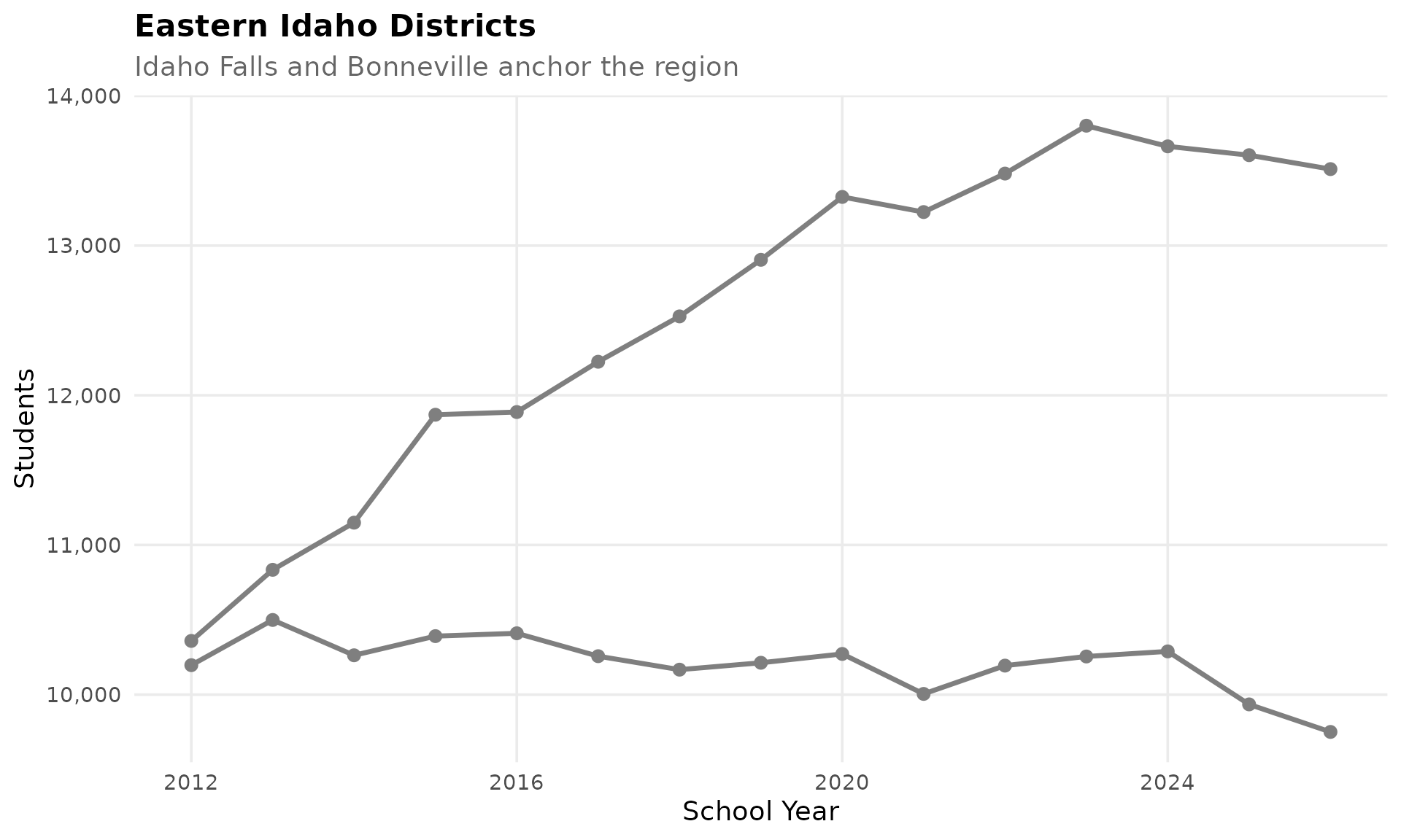
Session Info
sessionInfo()
#> R version 4.5.2 (2025-10-31)
#> Platform: x86_64-pc-linux-gnu
#> Running under: Ubuntu 24.04.3 LTS
#>
#> Matrix products: default
#> BLAS:   /usr/lib/x86_64-linux-gnu/openblas-pthread/libblas.so.3
#> LAPACK: /usr/lib/x86_64-linux-gnu/openblas-pthread/libopenblasp-r0.3.26.so;  LAPACK version 3.12.0
#>
#> locale:
#>  [1] LC_CTYPE=C.UTF-8       LC_NUMERIC=C           LC_TIME=C.UTF-8
#>  [4] LC_COLLATE=C.UTF-8     LC_MONETARY=C.UTF-8    LC_MESSAGES=C.UTF-8
#>  [7] LC_PAPER=C.UTF-8       LC_NAME=C              LC_ADDRESS=C
#> [10] LC_TELEPHONE=C         LC_MEASUREMENT=C.UTF-8 LC_IDENTIFICATION=C
#>
#> time zone: UTC
#> tzcode source: system (glibc)
#>
#> attached base packages:
#> [1] stats     graphics  grDevices utils     datasets  methods   base
#>
#> other attached packages:
#> [1] scales_1.4.0       dplyr_1.2.0        ggplot2_4.0.2      idschooldata_0.1.0
#>
#> loaded via a namespace (and not attached):
#>  [1] gtable_0.3.6       jsonlite_2.0.0     compiler_4.5.2     tidyselect_1.2.1
#>  [5] jquerylib_0.1.4    systemfonts_1.3.2  textshaping_1.0.5  readxl_1.4.5
#>  [9] yaml_2.3.12        fastmap_1.2.0      R6_2.6.1           labeling_0.4.3
#> [13] generics_0.1.4     curl_7.0.0         knitr_1.51         tibble_3.3.1
#> [17] desc_1.4.3         bslib_0.10.0       pillar_1.11.1      RColorBrewer_1.1-3
#> [21] rlang_1.1.7        utf8_1.2.6         cachem_1.1.0       xfun_0.56
#> [25] fs_1.6.7           sass_0.4.10        S7_0.2.1           cli_3.6.5
#> [29] pkgdown_2.2.0      withr_3.0.2        magrittr_2.0.4     digest_0.6.39
#> [33] grid_4.5.2         rappdirs_0.3.4     lifecycle_1.0.5    vctrs_0.7.1
#> [37] evaluate_1.0.5     glue_1.8.0         cellranger_1.1.0   farver_2.1.2
#> [41] codetools_0.2-20   ragg_1.5.1         httr_1.4.8         rmarkdown_2.30
#> [45] purrr_1.2.1        tools_4.5.2        pkgconfig_2.0.3    htmltools_0.5.9