Illinois Assessment Data: A Comprehensive Guide
Source:vignettes/illinois-assessment.Rmd
illinois-assessment.RmdIllinois Assessment Overview
Illinois has had three major state assessment systems over the past two decades:
| Era | Assessment | Years | Key Features |
|---|---|---|---|
| ISAT | Illinois Standards Achievement Test | 2006-2014 | Reading, Math, Science |
| PARCC | Partnership for Assessment of Readiness | 2015-2018 | Common Core aligned |
| IAR | Illinois Assessment of Readiness | 2019-present | PARCC successor |
Note: 2020 had no statewide testing due to the COVID-19 pandemic.
1. Steady Math Proficiency During PARCC Era (2016-2017)
Illinois showed steady math proficiency during the PARCC era, with district-average math proficiency holding at about 40%.
# Compare PARCC 2016 to PARCC 2017 at district level
parcc_2016 <- fetch_assessment(2016, use_cache = TRUE)
parcc_2017 <- fetch_assessment(2017, use_cache = TRUE)

# State average proficiency (Math)
parcc_2016_dist <- parcc_2016 %>%
  filter(is_district, subject == "Math") %>%
  summarize(
    year = 2016,
    assessment = "PARCC",
    mean_proficiency = mean(pct_proficient, na.rm = TRUE)
  )

parcc_2017_dist <- parcc_2017 %>%
  filter(is_district, subject == "Math") %>%
  summarize(
    year = 2017,
    assessment = "PARCC",
    mean_proficiency = mean(pct_proficient, na.rm = TRUE)
  )

stopifnot(nrow(parcc_2016_dist) > 0, nrow(parcc_2017_dist) > 0)
print(bind_rows(parcc_2016_dist, parcc_2017_dist))
## year assessment mean_proficiency
## 1 2016 PARCC 40.39410
## 2 2017 PARCC 40.513482. Chicago Public Schools Serves 1 in 5 Illinois Students
Chicago Public Schools (CPS) is by far the largest district in Illinois, serving roughly 20% of all public school students in the state.
# Get 2017 assessment data
assess_2017 <- fetch_assessment(2017, use_cache = TRUE)

# Find CPS (City of Chicago SD 299)
cps <- assess_2017 %>%
  filter(rcdts == "150162990250000", subject == "ELA") %>%
  select(district_name, pct_proficient)

stopifnot(nrow(cps) > 0)
print(cps)
## district_name pct_proficient
## 1 City of Chicago SD 299 31.63. District Proficiency Ranges from 0% to Over 90%
Illinois districts show enormous variation in assessment outcomes, reflecting the state’s economic and demographic diversity.
# ELA proficiency range across districts
ela_districts <- assess_2017 %>%
  filter(is_district, subject == "ELA")

ela_summary <- ela_districts %>%
  summarize(
    n_districts = n(),
    min_proficiency = min(pct_proficient, na.rm = TRUE),
    median_proficiency = median(pct_proficient, na.rm = TRUE),
    mean_proficiency = mean(pct_proficient, na.rm = TRUE),
    max_proficiency = max(pct_proficient, na.rm = TRUE)
  )

stopifnot(nrow(ela_summary) > 0)
print(ela_summary)
## n_districts min_proficiency median_proficiency mean_proficiency
## 1 712 0 36.25 37.69101
## max_proficiency
## 1 92.34. Top 10 Highest-Performing Districts in ELA
The highest-performing districts in ELA include a mix of small rural districts and affluent suburban districts.
top_ela <- assess_2017 %>%
  filter(is_district, subject == "ELA") %>%
  arrange(desc(pct_proficient)) %>%
  select(district_name, city, pct_proficient) %>%
  head(10)

stopifnot(nrow(top_ela) > 0)
print(top_ela)
## district_name city pct_proficient
## 1 Lisbon CCSD 90 Newark 92.3
## 2 St Elmo CUSD 202 Saint Elmo 83.4
## 3 Northbrook/Glenview SD 30 Northbrook 81.3
## 4 Northbrook ESD 27 Northbrook 81.0
## 5 Lowpoint-Washburn CUSD 21 Washburn 81.0
## 6 Oak Grove SD 68 Libertyville 80.4
## 7 Grant Park CUSD 6 Grant Park 80.0
## 8 Gower SD 62 Burr Ridge 79.6
## 9 Deerfield SD 109 Deerfield 79.5
## 10 Tremont CUSD 702 Tremont 78.75. Bottom 10 Districts in ELA Face Significant Challenges
Districts with the lowest proficiency rates often face concentrated poverty and other systemic challenges.
bottom_ela <- assess_2017 %>%
  filter(is_district, subject == "ELA", pct_proficient > 0) %>%
  arrange(pct_proficient) %>%
  select(district_name, city, pct_proficient) %>%
  head(10)

stopifnot(nrow(bottom_ela) > 0)
print(bottom_ela)
## district_name city pct_proficient
## 1 V I T CUSD 2 Table Grove 4.2
## 2 Cairo USD 1 Cairo 4.2
## 3 Pleasant Hill CUSD 3 Pleasant Hill 4.5
## 4 DeSoto Cons SD 86 De Soto 4.5
## 5 Cahokia CUSD 187 Cahokia 5.3
## 6 CCSD 168 Sauk Village 5.4
## 7 South Holland SD 151 Phoenix 5.7
## 8 Hoover-Schrum Memorial SD 157 Calumet City 6.2
## 9 Hardin County CUSD 1 Elizabethtown 6.8
## 10 Madison CUSD 12 Madison 7.16. Math Proficiency Slightly Higher Than ELA in Illinois
Across Illinois, district-average math proficiency (40.5%) slightly exceeds ELA proficiency (37.7%) on the 2017 PARCC assessment.
# Compare ELA and Math at district level
ela_math <- assess_2017 %>%
  filter(is_district) %>%
  select(rcdts, district_name, subject, pct_proficient) %>%
  pivot_wider(names_from = subject, values_from = pct_proficient)

ela_math_summary <- ela_math %>%
  filter(!is.na(ELA) & !is.na(Math)) %>%
  summarize(
    n_districts = n(),
    mean_ela = mean(ELA, na.rm = TRUE),
    mean_math = mean(Math, na.rm = TRUE),
    ela_higher_count = sum(ELA > Math, na.rm = TRUE)
  ) %>%
  mutate(ela_higher_pct = round(ela_higher_count / n_districts * 100, 1))

stopifnot(nrow(ela_math_summary) > 0)
print(ela_math_summary)
## # A tibble: 1 × 5
## n_districts mean_ela mean_math ela_higher_count ela_higher_pct
## <int> <dbl> <dbl> <int> <dbl>
## 1 712 37.7 40.5 254 35.7
ela_math_filtered <- ela_math %>% filter(!is.na(ELA) & !is.na(Math))
stopifnot(nrow(ela_math_filtered) > 0)

print(paste("Districts with both ELA and Math:", nrow(ela_math_filtered)))
## [1] "Districts with both ELA and Math: 712"
ggplot(ela_math_filtered, aes(x = Math, y = ELA)) +
  geom_point(alpha = 0.5) +
  geom_abline(slope = 1, intercept = 0, linetype = "dashed", color = "red") +
  labs(
    title = "ELA vs Math Proficiency by District (2017)",
    subtitle = "Points above the red line have higher ELA than Math",
    x = "Math Proficiency (%)",
    y = "ELA Proficiency (%)"
  ) +
  theme_minimal()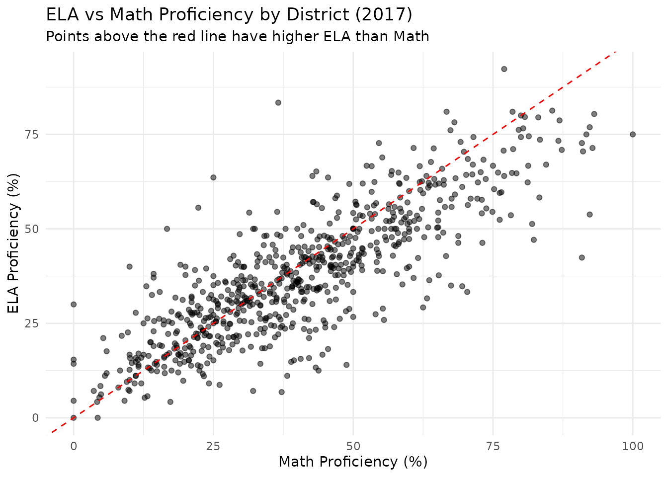
7. Top Counties by ELA Proficiency
Counties with 5+ districts vary widely in mean ELA proficiency. Rural Clinton County leads, while Cook County lags behind.
# Compare major counties
county_summary <- assess_2017 %>%
  filter(is_district, subject == "ELA") %>%
  group_by(county) %>%
  summarize(
    n_districts = n(),
    mean_proficiency = round(mean(pct_proficient, na.rm = TRUE), 1)
  ) %>%
  filter(n_districts >= 5) %>%
  arrange(desc(mean_proficiency))

stopifnot(nrow(county_summary) > 0)

# Show top counties
print(head(county_summary, 10))
## # A tibble: 10 × 3
## county n_districts mean_proficiency
## <chr> <int> <dbl>
## 1 Clinton 11 57.3
## 2 Wayne 5 53.6
## 3 Kendall 5 51.7
## 4 Woodford 8 50.1
## 5 Grundy 5 48.8
## 6 Effingham 5 48.2
## 7 Dupage 35 47.9
## 8 Morgan 5 46.9
## 9 Stephenson 5 45.5
## 10 Lake 37 44.98. Distribution of District Proficiency Rates
Most districts cluster around the statewide average, with long tails on both ends.
## [1] "Districts plotted: 712"
ggplot(ela_districts, aes(x = pct_proficient)) +
  geom_histogram(binwidth = 5, fill = "steelblue", color = "white") +
  geom_vline(
    xintercept = mean(ela_districts$pct_proficient, na.rm = TRUE),
    linetype = "dashed",
    color = "red"
  ) +
  labs(
    title = "Distribution of District ELA Proficiency (2017)",
    subtitle = "Red dashed line = statewide mean",
    x = "ELA Proficiency (%)",
    y = "Number of Districts"
  ) +
  theme_minimal()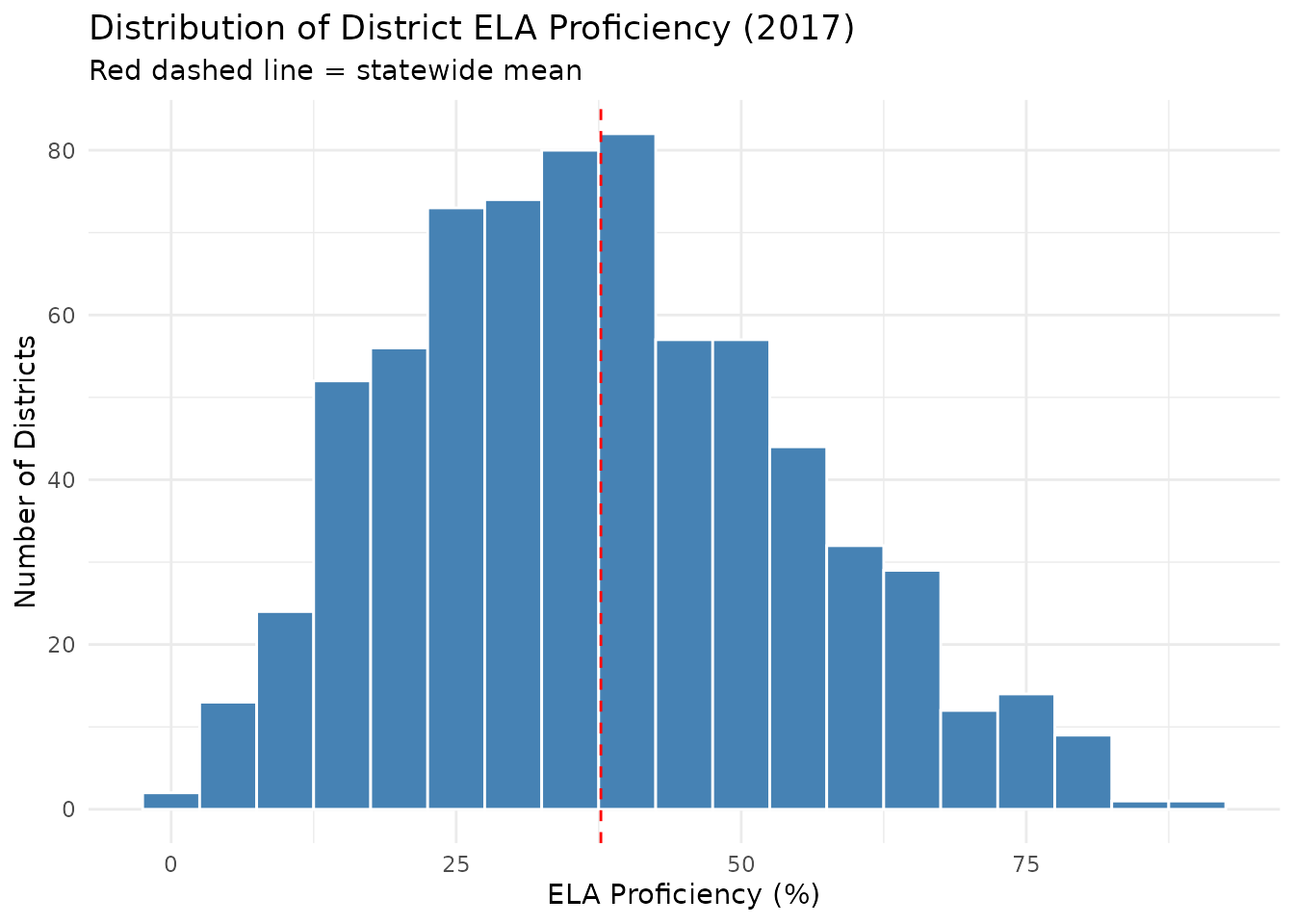
9. School-Level Data Shows Within-District Variation
Even within the same district, individual schools can vary widely in their assessment outcomes.
# Look at variation within major districts
school_variation <- assess_2017 %>%
  filter(is_school, subject == "ELA") %>%
  group_by(district_name) %>%
  summarize(
    n_schools = n(),
    min_prof = min(pct_proficient, na.rm = TRUE),
    max_prof = max(pct_proficient, na.rm = TRUE),
    range = max_prof - min_prof,
    sd = sd(pct_proficient, na.rm = TRUE)
  ) %>%
  filter(n_schools >= 10) %>%
  arrange(desc(range))

stopifnot(nrow(school_variation) > 0)
print(head(school_variation, 10))
## # A tibble: 3 × 6
## district_name n_schools min_prof max_prof range sd
## <chr> <int> <dbl> <dbl> <dbl> <dbl>
## 1 Lincoln Elem School 28 9.7 87.8 78.1 22.1
## 2 Washington Elem School 11 7 69.4 62.4 18.3
## 3 Jefferson Elem School 12 13.1 56 42.9 13.610. Year-Over-Year Changes: 2016 vs 2017
Comparing consecutive PARCC years reveals district-level changes in proficiency, controlling for the assessment system.
# Compare same district across consecutive PARCC years
parcc_2016_districts <- parcc_2016 %>%
  filter(is_district, subject == "Math") %>%
  select(rcdts, district_name, prof_2016 = pct_proficient)

parcc_2017_districts <- parcc_2017 %>%
  filter(is_district, subject == "Math") %>%
  select(rcdts, prof_2017 = pct_proficient)

comparison <- parcc_2016_districts %>%
  inner_join(parcc_2017_districts, by = "rcdts") %>%
  mutate(change = prof_2017 - prof_2016) %>%
  filter(!is.na(prof_2016) & !is.na(prof_2017))

comparison_summary <- comparison %>%
  summarize(
    n_districts = n(),
    mean_2016 = mean(prof_2016, na.rm = TRUE),
    mean_2017 = mean(prof_2017, na.rm = TRUE),
    mean_change = mean(change, na.rm = TRUE),
    pct_improved = mean(change > 0, na.rm = TRUE) * 100
  )

stopifnot(nrow(comparison_summary) > 0)
print(comparison_summary)
## n_districts mean_2016 mean_2017 mean_change pct_improved
## 1 702 40.41567 40.6651 0.2494302 49.0028511. Fetching Multiple Years of Data
Track trends over time by fetching multiple years.
# Fetch PARCC years (2016-2017)
years_data <- fetch_assessment_multi(c(2016, 2017), use_cache = TRUE)

# Track CPS over time
cps_trend <- years_data %>%
  filter(rcdts == "150162990250000") %>%
  select(end_year, subject, pct_proficient)

stopifnot(nrow(cps_trend) > 0)
print(cps_trend)
## end_year subject pct_proficient
## 1 2016 ELA 31.4
## 2 2016 Math 32.4
## 3 2017 ELA 31.6
## 4 2017 Math 30.912. Assessment Systems Changed Dramatically Over Time
Illinois has undergone significant assessment changes, making long-term comparisons challenging.
# Check available years and assessment systems
available <- get_available_assessment_years()

cat("Available years:\n")
## Available years:
print(available$years)## [1] 2006 2007 2008 2009 2010 2011 2012 2013 2014 2015 2016 2017 2018 2019 2021
## [16] 2022 2023 2024 2025
cat("\nAssessment systems by year:\n")##
## Assessment systems by year:## 2014 2017 2024
## "ISAT" "PARCC" "IAR"13. Working with Tidy vs Wide Format
The package supports both tidy (long) and wide data formats.
# Tidy format (default)
assess_tidy <- fetch_assessment(2017, tidy = TRUE, use_cache = TRUE)
print(head(assess_tidy[, c("district_name", "subject", "pct_proficient")], 4))
## district_name subject pct_proficient
## 1 Payson CUSD 1 ELA 32.5
## 3 Seymour Elementary School ELA 32.5
## 4 Liberty CUSD 2 ELA 61.7
## 6 Liberty Elementary School ELA 61.7
# Wide format
assess_wide <- fetch_assessment(2017, tidy = FALSE, use_cache = TRUE)
print(head(assess_wide[, c("district_name", "pct_proficient_ela", "pct_proficient_math")], 4))
## district_name pct_proficient_ela pct_proficient_math
## 1 Payson CUSD 1 32.5 30.2
## 2 Seymour High School NA NA
## 3 Seymour Elementary School 32.5 30.2
## 4 Liberty CUSD 2 61.7 64.714. Aggregation Flags Make Filtering Easy
The data includes boolean flags for quick filtering.
# Count by aggregation level
print(assess_2017 %>%
  group_by(aggregation_flag) %>%
  summarize(n = n()) %>%
  arrange(desc(n)))
## # A tibble: 2 × 2
## aggregation_flag n
## <chr> <int>
## 1 campus 4064
## 2 district 1424
# Use flags directly
state_data <- assess_2017 %>% filter(is_state)
district_data <- assess_2017 %>% filter(is_district)
school_data <- assess_2017 %>% filter(is_school)

cat("State rows:", nrow(state_data), "\n")
## State rows: 0## District rows: 1424## School rows: 406415. Data Quality: Most Districts Have Valid Data
The vast majority of districts report valid proficiency rates.
# Check data quality
quality_check <- assess_2017 %>%
  filter(is_district, subject == "ELA") %>%
  summarize(
    total_districts = n(),
    with_proficiency = sum(!is.na(pct_proficient)),
    valid_range = sum(pct_proficient >= 0 & pct_proficient <= 100, na.rm = TRUE),
    pct_valid = round(valid_range / total_districts * 100, 1)
  )

stopifnot(nrow(quality_check) > 0)
print(quality_check)
## total_districts with_proficiency valid_range pct_valid
## 1 712 712 712 100Data Notes
Data Source
Assessment data comes from the Illinois State Board of Education (ISBE) Report Card Data Library: - URL: https://www.isbe.net/ilreportcarddata - PARCC/IAR files include district and school-level proficiency rates - ISAT files include assessment performance by grade and subject
Session Info
## R version 4.5.2 (2025-10-31)
## Platform: x86_64-pc-linux-gnu
## Running under: Ubuntu 24.04.3 LTS
##
## Matrix products: default
## BLAS:   /usr/lib/x86_64-linux-gnu/openblas-pthread/libblas.so.3
## LAPACK: /usr/lib/x86_64-linux-gnu/openblas-pthread/libopenblasp-r0.3.26.so;  LAPACK version 3.12.0
##
## locale:
##  [1] LC_CTYPE=C.UTF-8       LC_NUMERIC=C           LC_TIME=C.UTF-8
##  [4] LC_COLLATE=C.UTF-8     LC_MONETARY=C.UTF-8    LC_MESSAGES=C.UTF-8
##  [7] LC_PAPER=C.UTF-8       LC_NAME=C              LC_ADDRESS=C
## [10] LC_TELEPHONE=C         LC_MEASUREMENT=C.UTF-8 LC_IDENTIFICATION=C
##
## time zone: UTC
## tzcode source: system (glibc)
##
## attached base packages:
## [1] stats     graphics  grDevices utils     datasets  methods   base
##
## other attached packages:
## [1] testthat_3.3.2     tidyr_1.3.2        ggplot2_4.0.2      dplyr_1.2.0
## [5] ilschooldata_0.1.0
##
## loaded via a namespace (and not attached):
##  [1] gtable_0.3.6       jsonlite_2.0.0     compiler_4.5.2     brio_1.1.5
##  [5] tidyselect_1.2.1   jquerylib_0.1.4    systemfonts_1.3.2  scales_1.4.0
##  [9] textshaping_1.0.5  readxl_1.4.5       yaml_2.3.12        fastmap_1.2.0
## [13] R6_2.6.1           labeling_0.4.3     generics_0.1.4     knitr_1.51
## [17] tibble_3.3.1       desc_1.4.3         downloader_0.4.1   bslib_0.10.0
## [21] pillar_1.11.1      RColorBrewer_1.1-3 rlang_1.1.7        utf8_1.2.6
## [25] cachem_1.1.0       xfun_0.56          fs_1.6.7           sass_0.4.10
## [29] S7_0.2.1           cli_3.6.5          pkgdown_2.2.0      withr_3.0.2
## [33] magrittr_2.0.4     digest_0.6.39      grid_4.5.2         rappdirs_0.3.4
## [37] lifecycle_1.0.5    vctrs_0.7.1        evaluate_1.0.5     glue_1.8.0
## [41] cellranger_1.1.0   farver_2.1.2       codetools_0.2-20   ragg_1.5.1
## [45] purrr_1.2.1        rmarkdown_2.30     tools_4.5.2        pkgconfig_2.0.3
## [49] htmltools_0.5.9