16 Insights from North Dakota School Enrollment Data
Source:vignettes/enrollment_hooks.Rmd
enrollment_hooks.Rmd
library(ndschooldata)
library(dplyr)
library(tidyr)
library(ggplot2)
theme_set(theme_minimal(base_size = 14))
North Dakota’s school enrollment tells a story of oil booms, suburban growth, and rural consolidation. This vignette visualizes the key insights from the ndschooldata package.
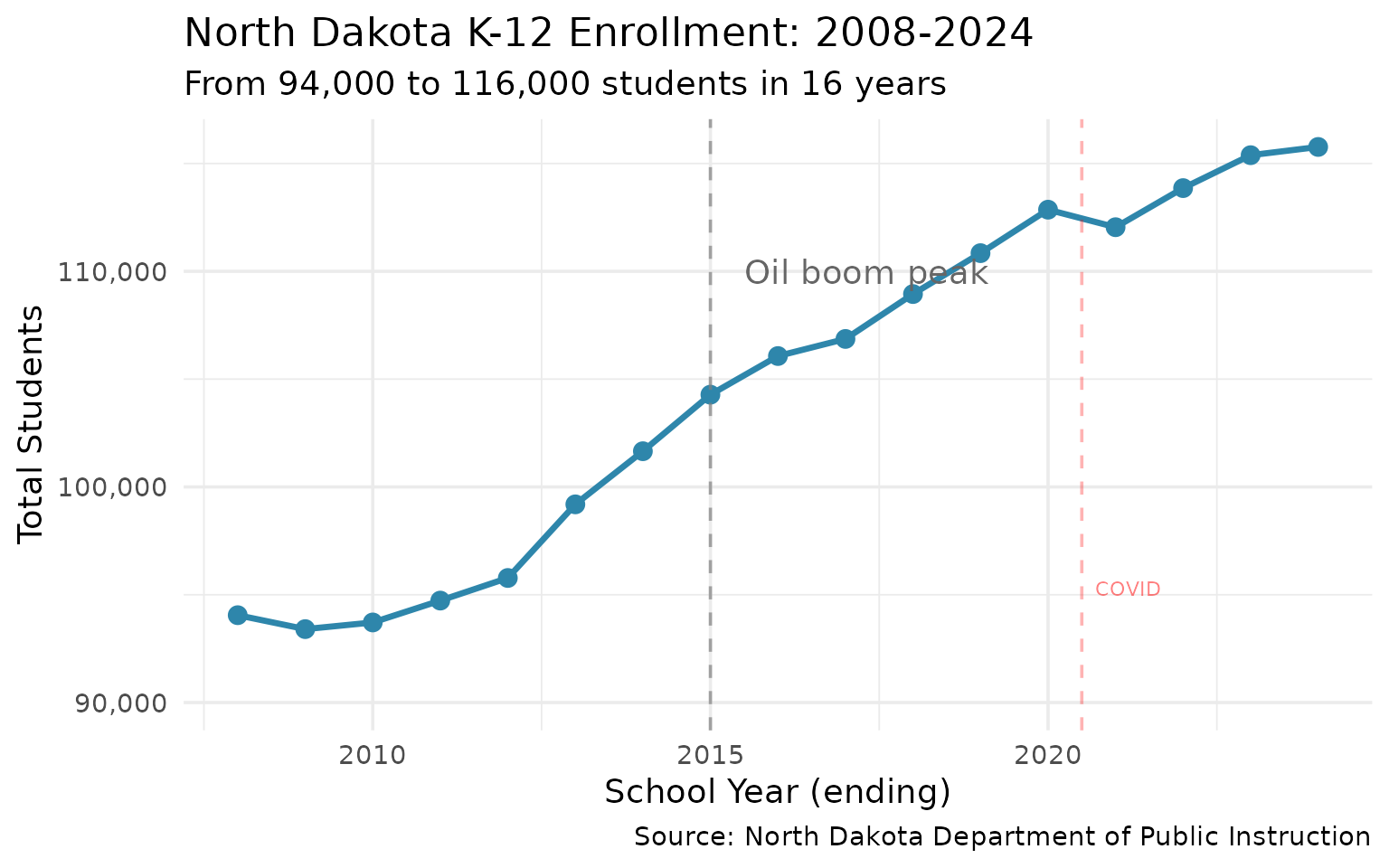
1. The Oil Boom Reshaped North Dakota Schools
Enrollment grew 23% from 2008 to 2024 as the Bakken brought families to the state.
enr <- tryCatch(
  fetch_enr_multi(2008:2024, use_cache = TRUE),
  error = function(e) {
    warning("Failed to fetch enrollment data: ", e$message)
    stop(e)
  }
)

statewide <- enr %>%
  filter(is_state, subgroup == "total_enrollment", grade_level == "TOTAL") %>%
  select(end_year, n_students)

stopifnot(nrow(statewide) > 0)
statewide
#>    end_year n_students
#> 1      2008      94052
#> 2      2009      93406
#> 3      2010      93715
#> 4      2011      94729
#> 5      2012      95778
#> 6      2013      99192
#> 7      2014     101656
#> 8      2015     104278
#> 9      2016     106070
#> 10     2017     106863
#> 11     2018     108945
#> 12     2019     110842
#> 13     2020     112858
#> 14     2021     112045
#> 15     2022     113858
#> 16     2023     115385
#> 17     2024     115767
ggplot(statewide, aes(x = end_year, y = n_students)) +
  geom_line(color = "#2E86AB", linewidth = 1.2) +
  geom_point(color = "#2E86AB", size = 3) +
  geom_vline(xintercept = 2015, linetype = "dashed", color = "gray50", alpha = 0.7) +
  annotate("text", x = 2015.5, y = max(statewide$n_students) * 0.95,
           label = "Oil boom peak", hjust = 0, color = "gray40") +
  geom_vline(xintercept = 2020.5, linetype = "dashed", color = "red", alpha = 0.3) +
  annotate("text", x = 2020.7, y = min(statewide$n_students) * 1.02,
           label = "COVID", hjust = 0, color = "red", alpha = 0.5, size = 3) +
  scale_y_continuous(labels = scales::comma, limits = c(90000, NA)) +
  labs(
    title = "North Dakota K-12 Enrollment: 2008-2024",
    subtitle = "From 94,000 to 116,000 students in 16 years",
    x = "School Year (ending)",
    y = "Total Students",
    caption = "Source: North Dakota Department of Public Instruction"
  )
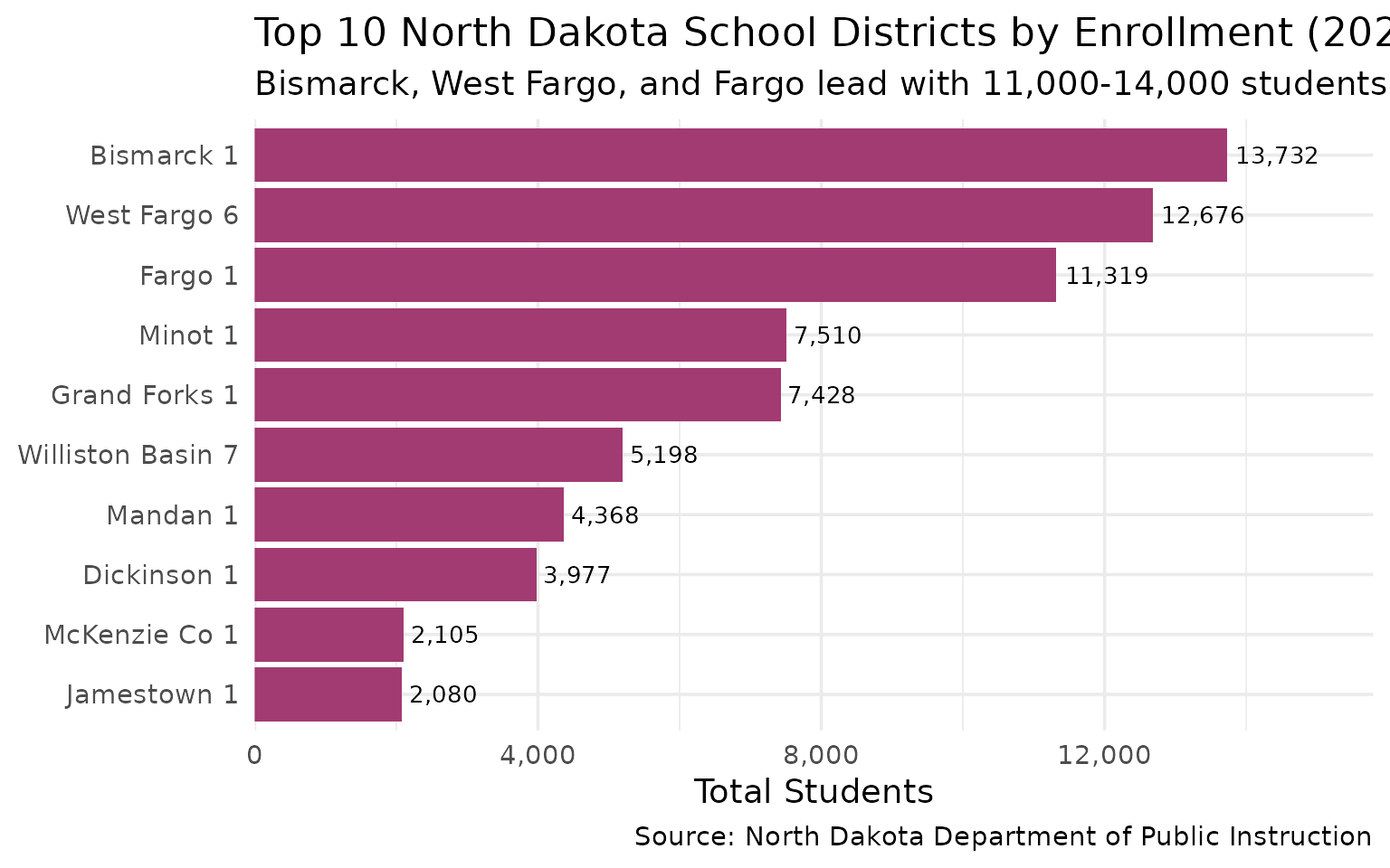
2. Bismarck Leads the State in Enrollment
The capital city edges out West Fargo and Fargo as the state’s largest district.
enr_2024 <- tryCatch(
  fetch_enr(2024, use_cache = TRUE),
  error = function(e) {
    warning("Failed to fetch 2024 enrollment data: ", e$message)
    stop(e)
  }
)

top_districts <- enr_2024 %>%
  filter(is_district, subgroup == "total_enrollment", grade_level == "TOTAL") %>%
  arrange(desc(n_students)) %>%
  head(10) %>%
  select(district_name, n_students) %>%
  mutate(district_name = gsub(" Public Schools| School District", "", district_name))

stopifnot(nrow(top_districts) > 0)
top_districts
#>        district_name n_students
#> 1         Bismarck 1      13732
#> 2       West Fargo 6      12676
#> 3            Fargo 1      11319
#> 4            Minot 1       7510
#> 5      Grand Forks 1       7428
#> 6  Williston Basin 7       5198
#> 7           Mandan 1       4368
#> 8        Dickinson 1       3977
#> 9      McKenzie Co 1       2105
#> 10       Jamestown 1       2080
ggplot(top_districts, aes(x = reorder(district_name, n_students), y = n_students)) +
  geom_col(fill = "#A23B72") +
  geom_text(aes(label = scales::comma(n_students)), hjust = -0.1, size = 3.5) +
  coord_flip() +
  scale_y_continuous(labels = scales::comma, expand = expansion(mult = c(0, 0.15))) +
  labs(
    title = "Top 10 North Dakota School Districts by Enrollment (2024)",
    subtitle = "Bismarck, West Fargo, and Fargo lead with 11,000-14,000 students each",
    x = NULL,
    y = "Total Students",
    caption = "Source: North Dakota Department of Public Instruction"
  )
3. West Fargo Doubled in Size Since 2008
The Fargo suburb is one of the fastest-growing districts in the country.
growth_districts <- enr %>%
  filter(is_district, subgroup == "total_enrollment", grade_level == "TOTAL",
         grepl("West Fargo|Fargo|Bismarck|Williston|Minot", district_name)) %>%
  mutate(district_name = trimws(gsub(" Public Schools| School District| Basin| [0-9]+$", "", district_name))) %>%
  filter(district_name %in% c("Fargo", "West Fargo", "Bismarck", "Williston", "Minot"))

stopifnot(nrow(growth_districts) > 0)

# Normalize to 2008 baseline
growth_indexed <- growth_districts %>%
  group_by(district_name) %>%
  mutate(baseline = n_students[end_year == min(end_year)],
         index = n_students / baseline * 100) %>%
  ungroup()

growth_indexed %>%
  filter(end_year %in% c(2008, 2024)) %>%
  select(district_name, end_year, n_students, index)
#> # A tibble: 10 × 4
#>    district_name end_year n_students index
#>    <chr>            <int>      <dbl> <dbl>
#>  1 Bismarck          2008      10638  100
#>  2 Fargo             2008      10493  100
#>  3 West Fargo        2008       6179  100
#>  4 Minot             2008       6243  100
#>  5 Williston         2008       2110  100
#>  6 Bismarck          2024      13732  129.
#>  7 Fargo             2024      11319  108.
#>  8 West Fargo        2024      12676  205.
#>  9 Minot             2024       7510  120.
#> 10 Williston         2024       5198  246.
ggplot(growth_indexed, aes(x = end_year, y = index, color = district_name)) +
  geom_line(linewidth = 1) +
  geom_point(size = 2) +
  geom_hline(yintercept = 100, linetype = "dashed", color = "gray50") +
  geom_vline(xintercept = 2020.5, linetype = "dashed", color = "red", alpha = 0.3) +
  annotate("text", x = 2020.7, y = 105, label = "COVID", hjust = 0, color = "red", alpha = 0.5, size = 3) +
  scale_color_brewer(palette = "Set1") +
  labs(
    title = "District Growth Compared (Indexed to 2008 = 100)",
    subtitle = "West Fargo and Williston saw explosive growth; others held steady",
    x = "School Year (ending)",
    y = "Enrollment Index (2008 = 100)",
    color = "District",
    caption = "Source: North Dakota Department of Public Instruction"
  ) +
  theme(legend.position = "bottom")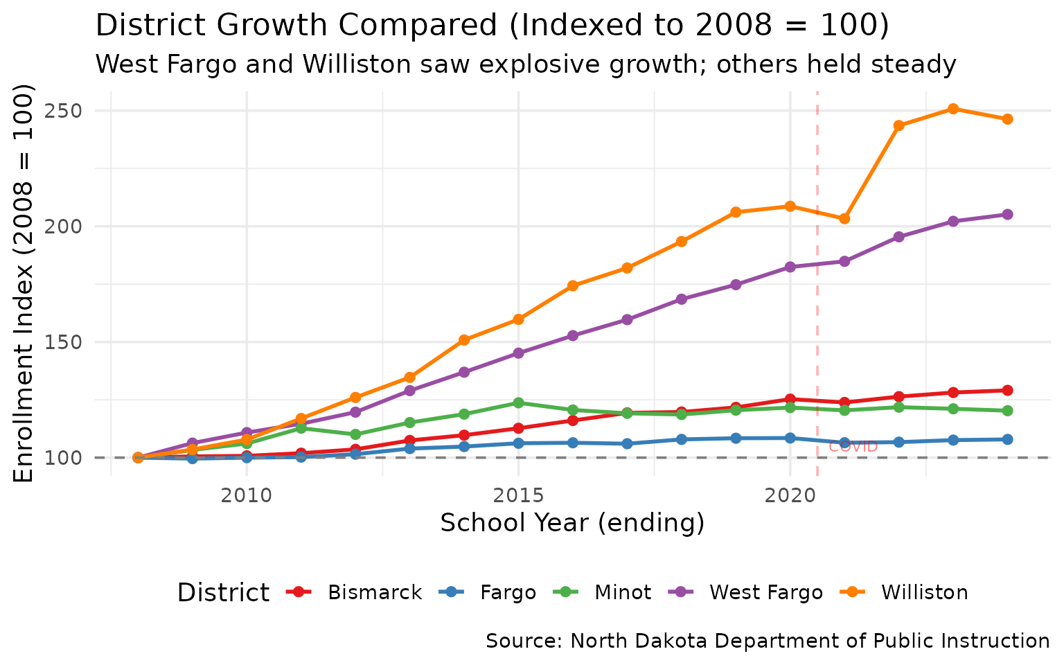
4. Kindergarten Enrollment Dropped 10% from Its Peak
The enrollment wave from the oil boom is aging out. Kindergarten peaked at 9,620 in 2020 and fell to 8,636 by 2024.
grade_levels <- enr %>%
  filter(is_state, subgroup == "total_enrollment") %>%
  mutate(level = case_when(
    grade_level %in% c("K", "01", "02", "03", "04", "05") ~ "Elementary (K-5)",
    grade_level %in% c("06", "07", "08") ~ "Middle (6-8)",
    grade_level %in% c("09", "10", "11", "12") ~ "High School (9-12)",
    TRUE ~ NA_character_
  )) %>%
  filter(!is.na(level)) %>%
  group_by(end_year, level) %>%
  summarize(total = sum(n_students, na.rm = TRUE), .groups = "drop")

stopifnot(nrow(grade_levels) > 0)
grade_levels %>% filter(end_year %in% c(2008, 2019, 2024)) %>% arrange(end_year, level)
#> # A tibble: 9 × 3
#>   end_year level              total
#>      <int> <chr>              <dbl>
#> 1     2008 Elementary (K-5)   40768
#> 2     2008 High School (9-12) 31492
#> 3     2008 Middle (6-8)       21792
#> 4     2019 Elementary (K-5)   53721
#> 5     2019 High School (9-12) 31430
#> 6     2019 Middle (6-8)       25691
#> 7     2024 Elementary (K-5)   54642
#> 8     2024 High School (9-12) 34556
#> 9     2024 Middle (6-8)       26569
ggplot(grade_levels, aes(x = end_year, y = total, fill = level)) +
  geom_area(alpha = 0.8) +
  geom_vline(xintercept = 2020.5, linetype = "dashed", color = "red", alpha = 0.3) +
  annotate("text", x = 2020.7, y = max(grade_levels$total) * 0.5,
           label = "COVID", hjust = 0, color = "red", alpha = 0.5, size = 3) +
  scale_fill_manual(values = c("Elementary (K-5)" = "#F18F01",
                               "Middle (6-8)" = "#C73E1D",
                               "High School (9-12)" = "#3C1642")) +
  scale_y_continuous(labels = scales::comma) +
  labs(
    title = "Enrollment by Grade Level: 2008-2024",
    subtitle = "Elementary grew from 2008-2023 but dipped in 2024; high school still growing",
    x = "School Year (ending)",
    y = "Total Students",
    fill = "Grade Level",
    caption = "Source: North Dakota Department of Public Instruction"
  ) +
  theme(legend.position = "bottom")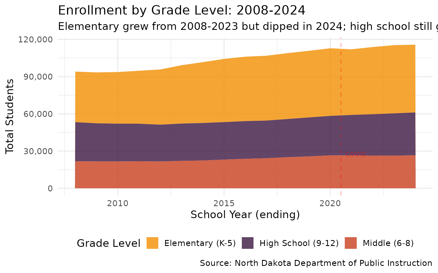
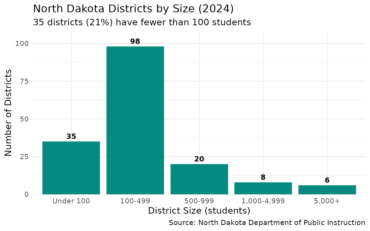
5. 35 Districts Have Under 100 Students
Tiny rural schools define the North Dakota landscape.
size_dist <- enr_2024 %>%
  filter(is_district, subgroup == "total_enrollment", grade_level == "TOTAL") %>%
  mutate(size_category = case_when(
    n_students < 100 ~ "Under 100",
    n_students < 500 ~ "100-499",
    n_students < 1000 ~ "500-999",
    n_students < 5000 ~ "1,000-4,999",
    TRUE ~ "5,000+"
  )) %>%
  mutate(size_category = factor(size_category,
                                levels = c("Under 100", "100-499", "500-999",
                                          "1,000-4,999", "5,000+"))) %>%
  count(size_category)

stopifnot(nrow(size_dist) > 0)
size_dist
#>   size_category  n
#> 1     Under 100 35
#> 2       100-499 98
#> 3       500-999 20
#> 4   1,000-4,999  8
#> 5        5,000+  6
ggplot(size_dist, aes(x = size_category, y = n)) +
  geom_col(fill = "#048A81") +
  geom_text(aes(label = n), vjust = -0.5, size = 4, fontface = "bold") +
  scale_y_continuous(expand = expansion(mult = c(0, 0.1))) +
  labs(
    title = "North Dakota Districts by Size (2024)",
    subtitle = "35 districts (21%) have fewer than 100 students",
    x = "District Size (students)",
    y = "Number of Districts",
    caption = "Source: North Dakota Department of Public Instruction"
  )
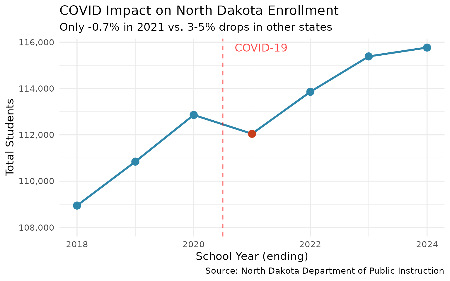
6. COVID Barely Dented North Dakota Enrollment (-0.7%)
Unlike other states, North Dakota saw only a small pandemic enrollment drop.
covid_years <- enr %>%
  filter(is_state, subgroup == "total_enrollment", grade_level == "TOTAL",
         end_year %in% 2018:2024) %>%
  select(end_year, n_students) %>%
  mutate(change = n_students - lag(n_students),
         pct_change = round(change / lag(n_students) * 100, 1))

stopifnot(nrow(covid_years) > 0)
covid_years
#>   end_year n_students change pct_change
#> 1     2018     108945     NA         NA
#> 2     2019     110842   1897        1.7
#> 3     2020     112858   2016        1.8
#> 4     2021     112045   -813       -0.7
#> 5     2022     113858   1813        1.6
#> 6     2023     115385   1527        1.3
#> 7     2024     115767    382        0.3
ggplot(covid_years, aes(x = end_year, y = n_students)) +
  geom_line(color = "#2E86AB", linewidth = 1.2) +
  geom_point(aes(color = end_year == 2021), size = 4) +
  geom_vline(xintercept = 2020.5, linetype = "dashed", color = "red", alpha = 0.5) +
  annotate("text", x = 2020.7, y = max(covid_years$n_students),
           label = "COVID-19", hjust = 0, color = "red", alpha = 0.7) +
  scale_color_manual(values = c("FALSE" = "#2E86AB", "TRUE" = "#C73E1D"), guide = "none") +
  scale_y_continuous(labels = scales::comma, limits = c(108000, NA)) +
  labs(
    title = "COVID Impact on North Dakota Enrollment",
    subtitle = "Only -0.7% in 2021 vs. 3-5% drops in other states",
    x = "School Year (ending)",
    y = "Total Students",
    caption = "Source: North Dakota Department of Public Instruction"
  )
7. Oil Counties vs. Traditional Farming Areas
The Bakken oil formation transformed Williams and McKenzie counties while agricultural areas stayed flat.
oil_districts <- enr %>%
  filter(is_district, subgroup == "total_enrollment", grade_level == "TOTAL",
         grepl("Williston|Watford|Tioga|Alexander|Dickinson|Mandan", district_name)) %>%
  mutate(region = case_when(
    grepl("Williston|Watford|Tioga|Alexander", district_name) ~ "Oil Counties",
    TRUE ~ "Traditional"
  )) %>%
  group_by(end_year, region) %>%
  summarize(total = sum(n_students, na.rm = TRUE), .groups = "drop")

stopifnot(nrow(oil_districts) > 0)
oil_districts %>% filter(end_year %in% c(2008, 2015, 2024))
#> # A tibble: 6 × 3
#>   end_year region       total
#>      <int> <chr>        <dbl>
#> 1     2008 Oil Counties  2412
#> 2     2008 Traditional   5629
#> 3     2015 Oil Counties  4035
#> 4     2015 Traditional   6879
#> 5     2024 Oil Counties  6052
#> 6     2024 Traditional   8345
ggplot(oil_districts, aes(x = end_year, y = total, color = region)) +
  geom_line(linewidth = 1.2) +
  geom_point(size = 2) +
  geom_vline(xintercept = 2020.5, linetype = "dashed", color = "red", alpha = 0.3) +
  annotate("text", x = 2020.7, y = min(oil_districts$total) * 1.05,
           label = "COVID", hjust = 0, color = "red", alpha = 0.5, size = 3) +
  scale_color_manual(values = c("Oil Counties" = "#E63946", "Traditional" = "#457B9D")) +
  scale_y_continuous(labels = scales::comma) +
  labs(
    title = "Oil Boom Counties vs. Traditional Areas",
    subtitle = "Williams/McKenzie oil counties surged while Dickinson/Mandan held steady",
    x = "School Year (ending)",
    y = "Combined Enrollment",
    color = "Region",
    caption = "Source: North Dakota Department of Public Instruction"
  ) +
  theme(legend.position = "bottom")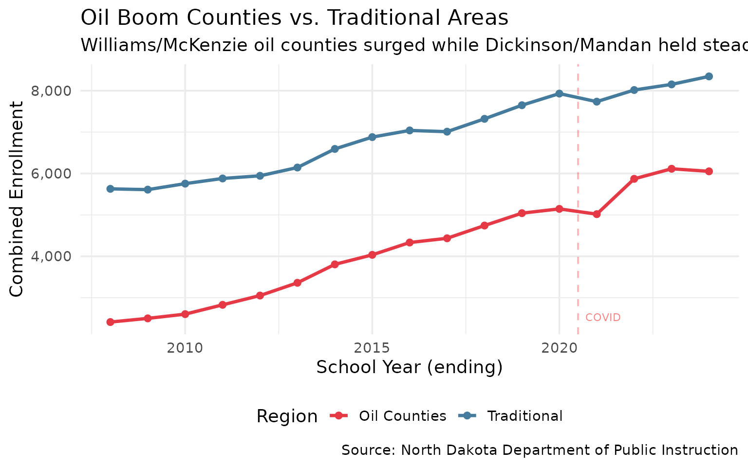
8. Bismarck: Steady Growth as State Capital
While West Fargo doubled in size, Bismarck’s enrollment has grown steadily without the volatility.
bismarck_growth <- enr %>%
  filter(is_district, subgroup == "total_enrollment", grade_level == "TOTAL",
         grepl("Bismarck|Fargo|West Fargo", district_name)) %>%
  mutate(district_name = trimws(gsub(" Public Schools| School District| [0-9]+$", "", district_name))) %>%
  filter(district_name %in% c("Bismarck", "Fargo", "West Fargo")) %>%
  group_by(district_name) %>%
  mutate(yoy_change = (n_students - lag(n_students)) / lag(n_students) * 100) %>%
  ungroup() %>%
  filter(!is.na(yoy_change))

stopifnot(nrow(bismarck_growth) > 0)
bismarck_growth %>%
  group_by(district_name) %>%
  summarize(avg_yoy = round(mean(yoy_change, na.rm = TRUE), 2),
            max_yoy = round(max(yoy_change, na.rm = TRUE), 2),
            min_yoy = round(min(yoy_change, na.rm = TRUE), 2))
#> # A tibble: 3 × 4
#>   district_name avg_yoy max_yoy min_yoy
#>   <chr>           <dbl>   <dbl>   <dbl>
#> 1 Bismarck         1.62    3.72   -1.16
#> 2 Fargo            0.48    2.39   -1.87
#> 3 West Fargo       4.61    7.78    1.33
ggplot(bismarck_growth, aes(x = end_year, y = yoy_change, color = district_name)) +
  geom_line(linewidth = 1) +
  geom_point(size = 2) +
  geom_hline(yintercept = 0, linetype = "dashed", color = "gray50") +
  geom_vline(xintercept = 2020.5, linetype = "dashed", color = "red", alpha = 0.3) +
  annotate("text", x = 2020.7, y = max(bismarck_growth$yoy_change) * 0.9,
           label = "COVID", hjust = 0, color = "red", alpha = 0.5, size = 3) +
  scale_color_manual(values = c("Bismarck" = "#1D3557", "Fargo" = "#E63946", "West Fargo" = "#A8DADC")) +
  labs(
    title = "Year-over-Year Enrollment Change: Big Three Districts",
    subtitle = "Bismarck grows steadily; West Fargo shows boom-era volatility",
    x = "School Year (ending)",
    y = "Percent Change from Previous Year",
    color = "District",
    caption = "Source: North Dakota Department of Public Instruction"
  ) +
  theme(legend.position = "bottom")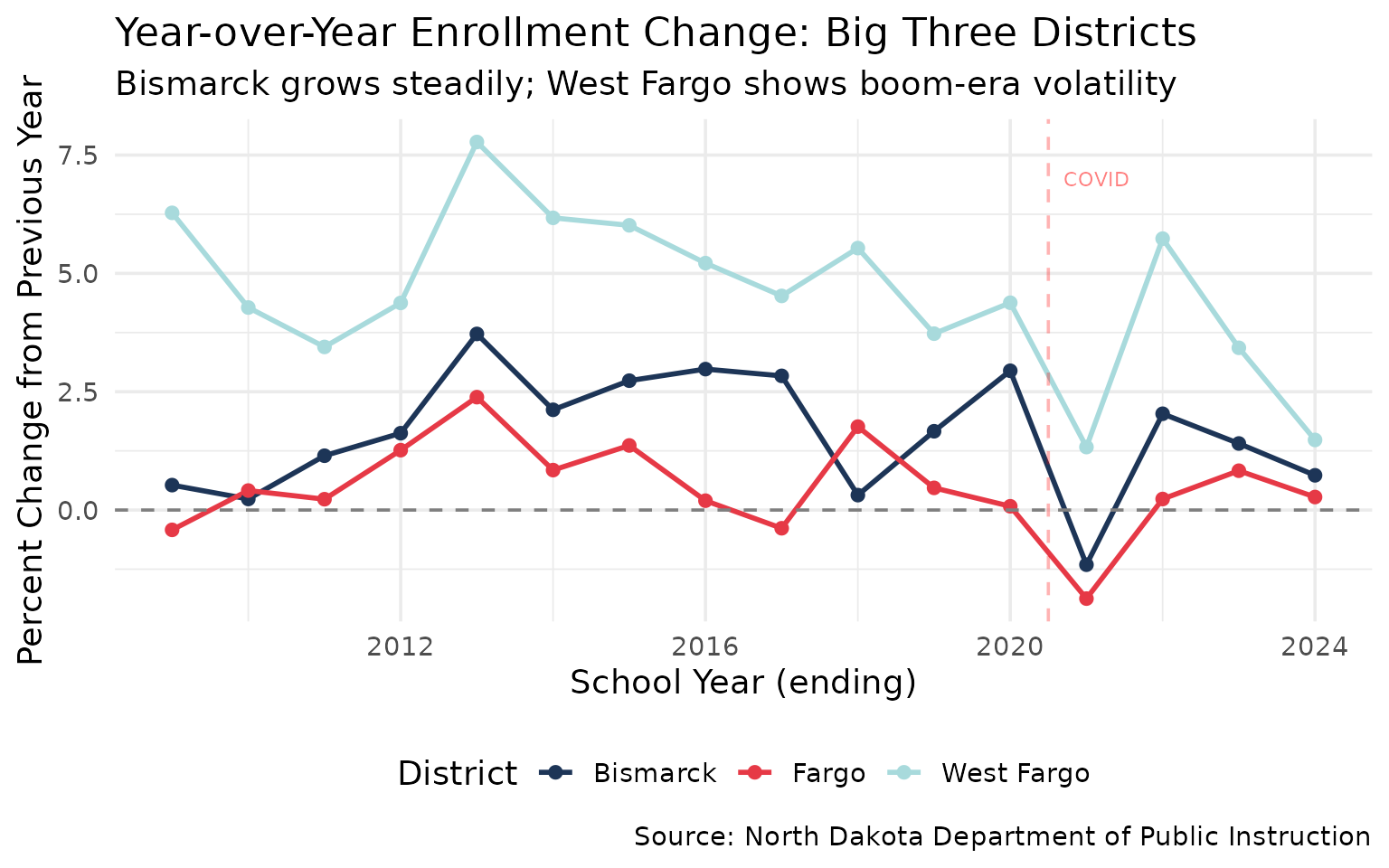
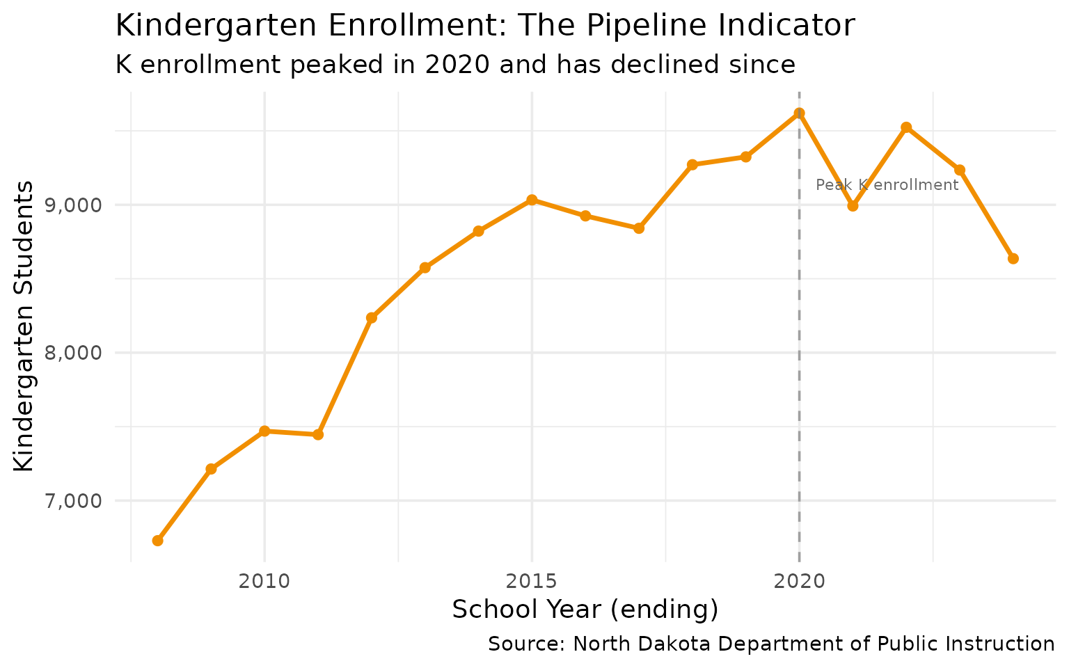
9. Kindergarten as a Leading Indicator
Kindergarten enrollment predicts total enrollment 12 years later. The recent K decline signals future challenges.
k_vs_total <- enr %>%
  filter(is_state, subgroup == "total_enrollment") %>%
  filter(grade_level %in% c("K", "TOTAL")) %>%
  select(end_year, grade_level, n_students) %>%
  pivot_wider(names_from = grade_level, values_from = n_students) %>%
  rename(kindergarten = K, total = TOTAL) %>%
  mutate(k_pct = kindergarten / total * 100)

stopifnot(nrow(k_vs_total) > 0)
k_vs_total %>% select(end_year, kindergarten, k_pct)
#> # A tibble: 17 × 3
#>    end_year kindergarten k_pct
#>       <int>        <dbl> <dbl>
#>  1     2008         6729  7.15
#>  2     2009         7214  7.72
#>  3     2010         7470  7.97
#>  4     2011         7446  7.86
#>  5     2012         8236  8.60
#>  6     2013         8575  8.64
#>  7     2014         8822  8.68
#>  8     2015         9033  8.66
#>  9     2016         8925  8.41
#> 10     2017         8841  8.27
#> 11     2018         9271  8.51
#> 12     2019         9324  8.41
#> 13     2020         9620  8.52
#> 14     2021         8992  8.03
#> 15     2022         9524  8.36
#> 16     2023         9235  8.00
#> 17     2024         8636  7.46
ggplot(k_vs_total, aes(x = end_year)) +
  geom_line(aes(y = kindergarten), color = "#F18F01", linewidth = 1.2) +
  geom_point(aes(y = kindergarten), color = "#F18F01", size = 2) +
  geom_vline(xintercept = 2020, linetype = "dashed", color = "gray50", alpha = 0.7) +
  annotate("text", x = 2020.3, y = max(k_vs_total$kindergarten, na.rm = TRUE) * 0.95,
           label = "Peak K enrollment", hjust = 0, color = "gray40", size = 3) +
  scale_y_continuous(labels = scales::comma) +
  labs(
    title = "Kindergarten Enrollment: The Pipeline Indicator",
    subtitle = "K enrollment peaked in 2020 and has declined since",
    x = "School Year (ending)",
    y = "Kindergarten Students",
    caption = "Source: North Dakota Department of Public Instruction"
  )
10. Grand Forks: Holding Steady While Others Surge
Grand Forks has stabilized while Fargo grew modestly and Minot plateaued after its oil-boom surge.
gf_trend <- enr %>%
  filter(is_district, subgroup == "total_enrollment", grade_level == "TOTAL",
         grepl("Grand Forks|Fargo|Minot", district_name)) %>%
  mutate(district_name = trimws(gsub(" Public Schools| School District| [0-9]+$", "", district_name))) %>%
  filter(district_name %in% c("Grand Forks", "Fargo", "Minot")) %>%
  group_by(district_name) %>%
  mutate(indexed = n_students / first(n_students) * 100) %>%
  ungroup()

stopifnot(nrow(gf_trend) > 0)
gf_trend %>% filter(end_year %in% c(2008, 2016, 2024)) %>% select(district_name, end_year, n_students, indexed)
#> # A tibble: 9 × 4
#>   district_name end_year n_students indexed
#>   <chr>            <int>      <dbl>   <dbl>
#> 1 Fargo             2008      10493    100
#> 2 Grand Forks       2008       7192    100
#> 3 Minot             2008       6243    100
#> 4 Fargo             2016      11167    106.
#> 5 Grand Forks       2016       7264    101.
#> 6 Minot             2016       7529    121.
#> 7 Fargo             2024      11319    108.
#> 8 Grand Forks       2024       7428    103.
#> 9 Minot             2024       7510    120.
ggplot(gf_trend, aes(x = end_year, y = indexed, color = district_name)) +
  geom_line(linewidth = 1.2) +
  geom_point(size = 2) +
  geom_hline(yintercept = 100, linetype = "dashed", color = "gray50") +
  geom_vline(xintercept = 2020.5, linetype = "dashed", color = "red", alpha = 0.3) +
  annotate("text", x = 2020.7, y = 98, label = "COVID", hjust = 0, color = "red", alpha = 0.5, size = 3) +
  scale_color_manual(values = c("Grand Forks" = "#2A9D8F", "Fargo" = "#E76F51", "Minot" = "#264653")) +
  labs(
    title = "Grand Forks, Fargo, and Minot: Growth Trajectories",
    subtitle = "Grand Forks has stabilized while Fargo grew modestly and Minot plateaued",
    x = "School Year (ending)",
    y = "Enrollment Index (2008 = 100)",
    color = "District",
    caption = "Source: North Dakota Department of Public Instruction"
  ) +
  theme(legend.position = "bottom")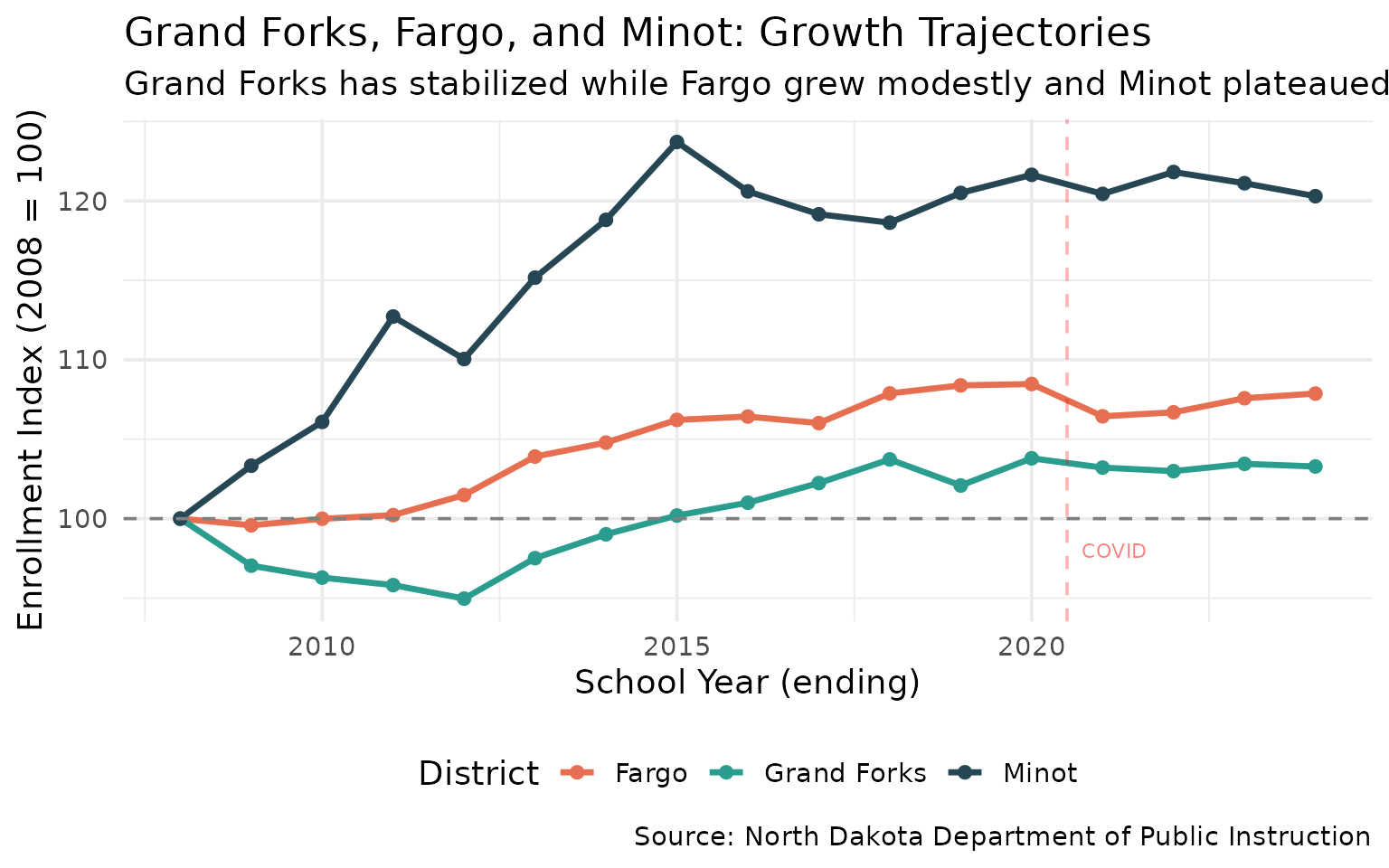
11. The Smallest Districts Are Getting Smaller
Rural consolidation continues as tiny districts shrink further.
# Track smallest districts over time
small_district_trend <- enr %>%
  filter(is_district, subgroup == "total_enrollment", grade_level == "TOTAL") %>%
  group_by(end_year) %>%
  summarize(
    under_50 = sum(n_students < 50, na.rm = TRUE),
    under_100 = sum(n_students < 100, na.rm = TRUE),
    under_200 = sum(n_students < 200, na.rm = TRUE),
    .groups = "drop"
  ) %>%
  pivot_longer(cols = starts_with("under"), names_to = "category", values_to = "count") %>%
  mutate(category = case_when(
    category == "under_50" ~ "Under 50 students",
    category == "under_100" ~ "Under 100 students",
    category == "under_200" ~ "Under 200 students"
  ))

stopifnot(nrow(small_district_trend) > 0)
small_district_trend %>% filter(end_year %in% c(2008, 2016, 2024)) %>% arrange(end_year, category)
#> # A tibble: 9 × 3
#>   end_year category           count
#>      <int> <chr>              <int>
#> 1     2008 Under 100 students    57
#> 2     2008 Under 200 students   100
#> 3     2008 Under 50 students     33
#> 4     2016 Under 100 students    39
#> 5     2016 Under 200 students    78
#> 6     2016 Under 50 students     20
#> 7     2024 Under 100 students    35
#> 8     2024 Under 200 students    73
#> 9     2024 Under 50 students     13
ggplot(small_district_trend, aes(x = end_year, y = count, fill = category)) +
  geom_area(alpha = 0.7, position = "identity") +
  geom_vline(xintercept = 2020.5, linetype = "dashed", color = "red", alpha = 0.3) +
  annotate("text", x = 2020.7, y = max(small_district_trend$count) * 0.95,
           label = "COVID", hjust = 0, color = "red", alpha = 0.5, size = 3) +
  scale_fill_manual(values = c("Under 50 students" = "#C73E1D",
                                "Under 100 students" = "#F18F01",
                                "Under 200 students" = "#048A81")) +
  labs(
    title = "Small Districts in North Dakota Over Time",
    subtitle = "The number of tiny districts remains high despite consolidation pressure",
    x = "School Year (ending)",
    y = "Number of Districts",
    fill = "Size Category",
    caption = "Source: North Dakota Department of Public Instruction"
  ) +
  theme(legend.position = "bottom")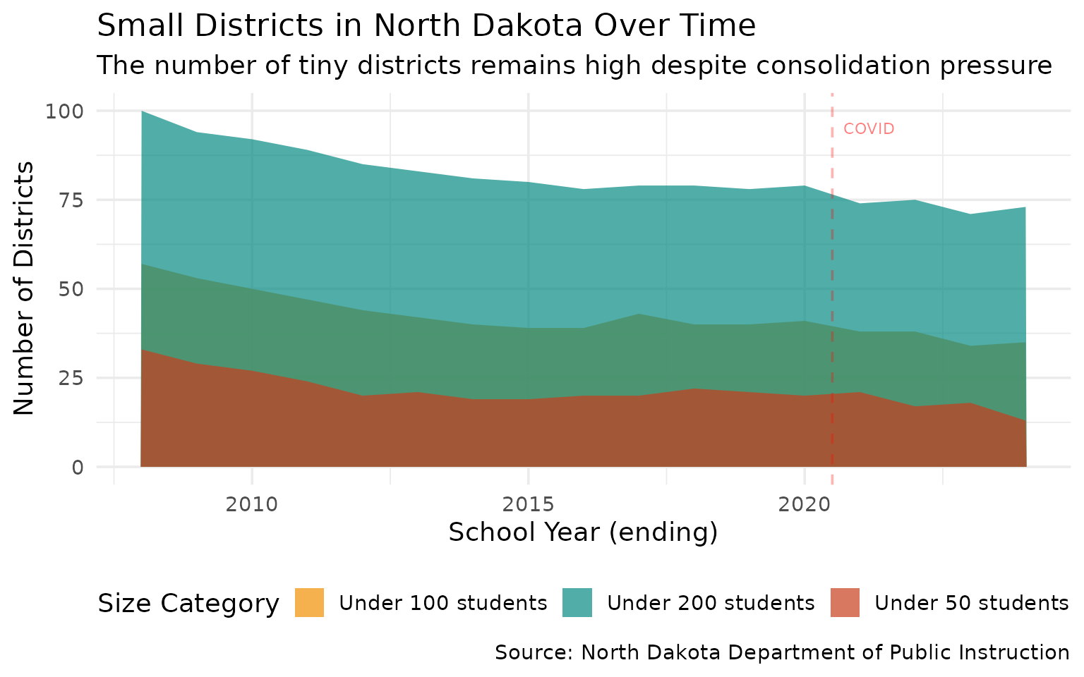
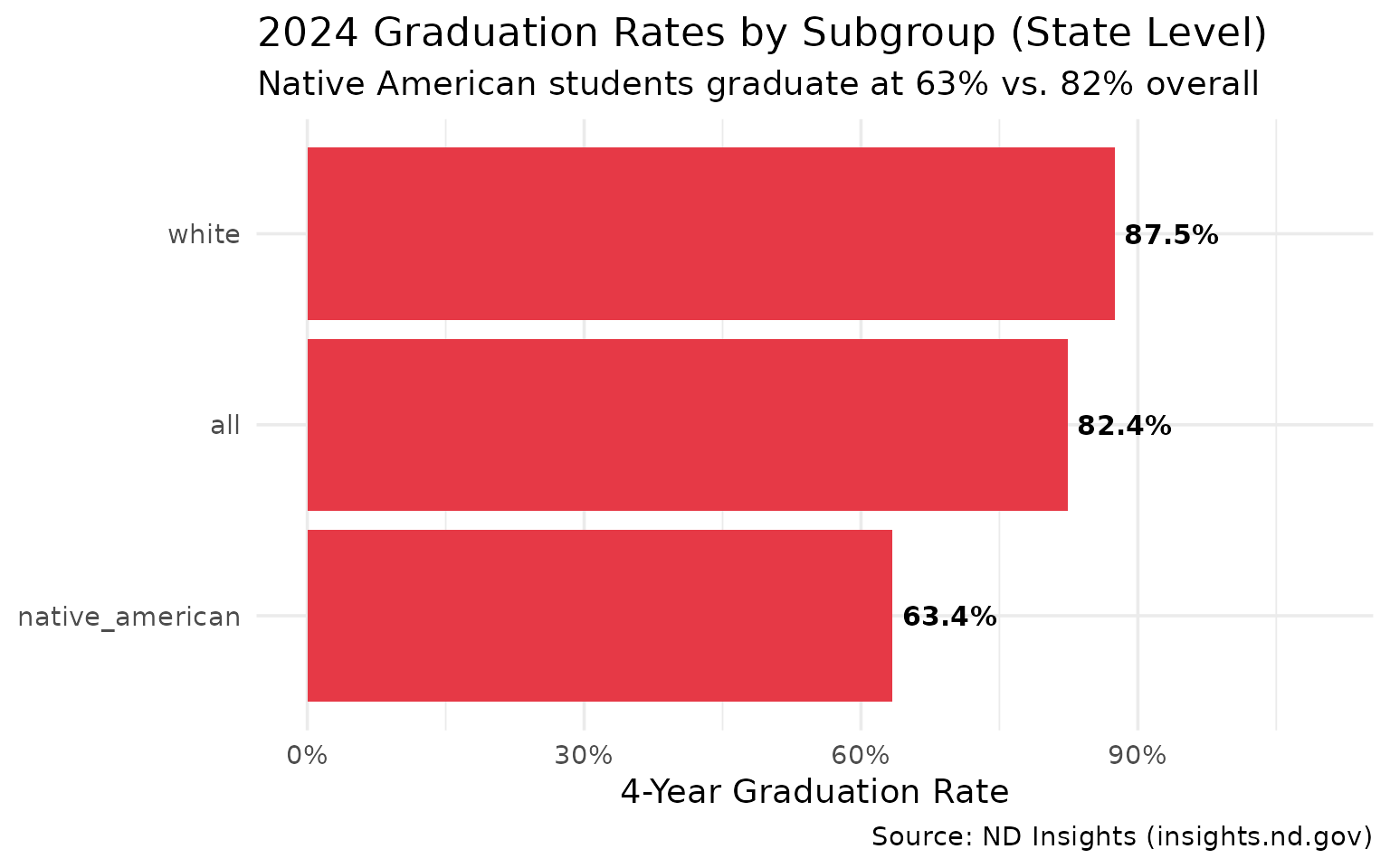
12. Native American Graduation Rates Lag State Average
Native American students face a 19-point graduation gap compared to the state average.
grad_2024 <- tryCatch(
  fetch_graduation(2024, use_cache = TRUE),
  error = function(e) {
    warning("Failed to fetch 2024 graduation data: ", e$message)
    stop(e)
  }
)

# Compare subgroups at state level
grad_subgroups <- grad_2024 %>%
  filter(is_state, subgroup %in% c("all", "native_american", "white", "low_income")) %>%
  select(subgroup, grad_rate, cohort_count, graduate_count) %>%
  arrange(desc(grad_rate))

stopifnot(nrow(grad_subgroups) > 0)
grad_subgroups
#> # A tibble: 3 × 4
#>   subgroup        grad_rate cohort_count graduate_count
#>   <chr>               <dbl>        <int>          <int>
#> 1 white               0.875         6420           5620
#> 2 all                 0.824         8681           7154
#> 3 native_american     0.634          939            595
ggplot(grad_subgroups, aes(x = reorder(subgroup, grad_rate), y = grad_rate)) +
  geom_col(fill = "#E63946") +
  geom_text(aes(label = paste0(round(grad_rate * 100, 1), "%")),
            hjust = -0.1, size = 4, fontface = "bold") +
  coord_flip() +
  scale_y_continuous(labels = scales::percent, limits = c(0, 1.1)) +
  labs(
    title = "2024 Graduation Rates by Subgroup (State Level)",
    subtitle = "Native American students graduate at 63% vs. 82% overall",
    x = NULL,
    y = "4-Year Graduation Rate",
    caption = "Source: ND Insights (insights.nd.gov)"
  )
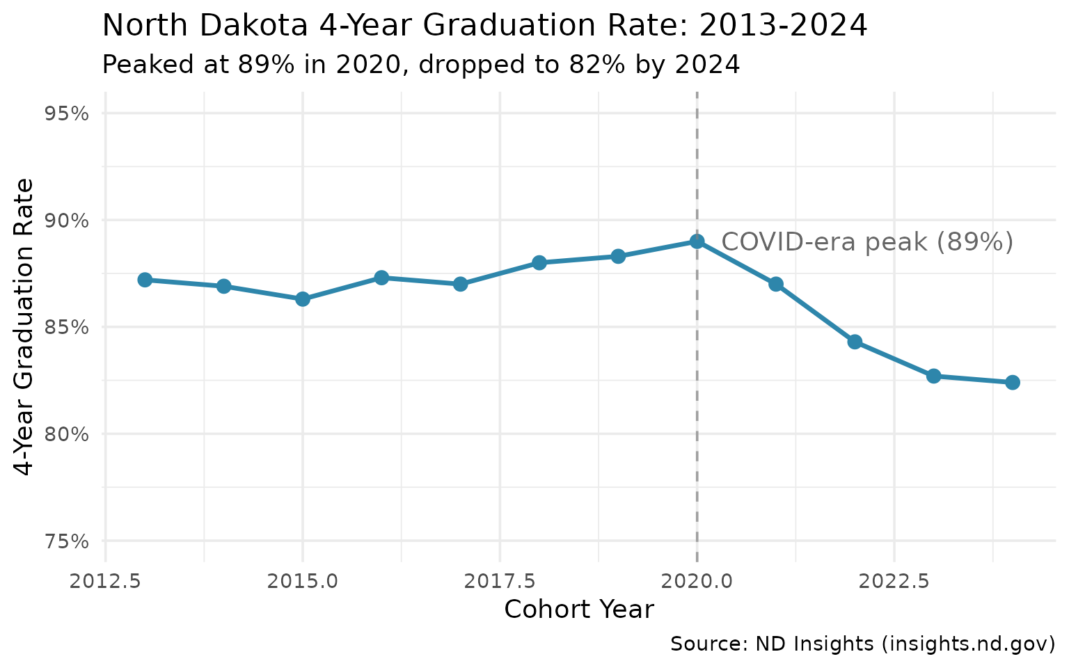
13. Graduation Rates Dropped 7 Points from Their Peak
The statewide graduation rate peaked at 89% in 2020 and has declined to 82% in four years.
grad_multi <- tryCatch(
  fetch_graduation_multi(2013:2024, use_cache = TRUE),
  error = function(e) {
    warning("Failed to fetch graduation data: ", e$message)
    stop(e)
  }
)

grad_trend <- grad_multi %>%
  filter(is_state, subgroup == "all") %>%
  select(end_year, grad_rate, cohort_count, graduate_count)

stopifnot(nrow(grad_trend) > 0)
grad_trend
#> # A tibble: 12 × 4
#>    end_year grad_rate cohort_count graduate_count
#>       <int>     <dbl>        <int>          <int>
#>  1     2013     0.872         7567           6598
#>  2     2014     0.869         7603           6609
#>  3     2015     0.863         7635           6589
#>  4     2016     0.873         7661           6687
#>  5     2017     0.87          7572           6588
#>  6     2018     0.88          7399           6512
#>  7     2019     0.883         7626           6730
#>  8     2020     0.89          7486           6660
#>  9     2021     0.87          7843           6825
#> 10     2022     0.843         8092           6823
#> 11     2023     0.827         8294           6863
#> 12     2024     0.824         8681           7154
ggplot(grad_trend, aes(x = end_year, y = grad_rate)) +
  geom_line(color = "#2E86AB", linewidth = 1.2) +
  geom_point(color = "#2E86AB", size = 3) +
  geom_vline(xintercept = 2020, linetype = "dashed", color = "gray50", alpha = 0.7) +
  annotate("text", x = 2020.3, y = 0.89, label = "COVID-era peak (89%)", hjust = 0, color = "gray40") +
  scale_y_continuous(labels = scales::percent, limits = c(0.75, 0.95)) +
  labs(
    title = "North Dakota 4-Year Graduation Rate: 2013-2024",
    subtitle = "Peaked at 89% in 2020, dropped to 82% by 2024",
    x = "Cohort Year",
    y = "4-Year Graduation Rate",
    caption = "Source: ND Insights (insights.nd.gov)"
  )
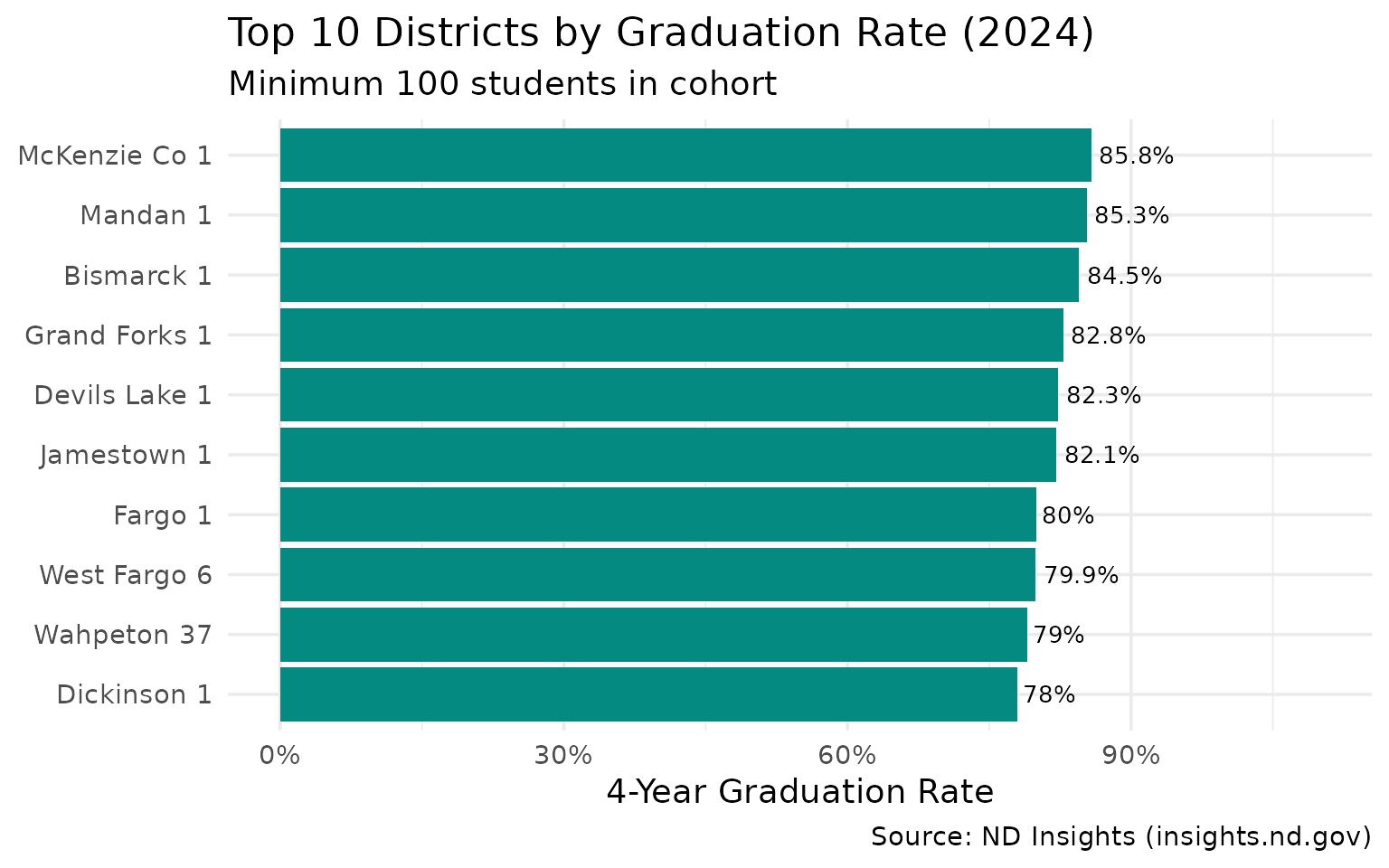
14. McKenzie County Leads in Graduation Rates
Among districts with 100+ student cohorts, the oil-country districts outperform the metro areas.
top_grad_districts <- grad_2024 %>%
  filter(is_district, subgroup == "all", cohort_count >= 100) %>%
  arrange(desc(grad_rate)) %>%
  head(10) %>%
  select(district_name, grad_rate, cohort_count, graduate_count) %>%
  mutate(district_name = gsub(" Public School.*| School District.*", "", district_name))

stopifnot(nrow(top_grad_districts) > 0)
top_grad_districts
#> # A tibble: 10 × 4
#>    district_name grad_rate cohort_count graduate_count
#>    <chr>             <dbl>        <int>          <int>
#>  1 McKenzie Co 1     0.858          106             91
#>  2 Mandan 1          0.853          334            285
#>  3 Bismarck 1        0.845         1057            893
#>  4 Grand Forks 1     0.828          599            496
#>  5 Devils Lake 1     0.823          130            107
#>  6 Jamestown 1       0.821          207            170
#>  7 Fargo 1           0.8            949            759
#>  8 West Fargo 6      0.799          884            706
#>  9 Wahpeton 37       0.79           119             94
#> 10 Dickinson 1       0.78           296            231
ggplot(top_grad_districts, aes(x = reorder(district_name, grad_rate), y = grad_rate)) +
  geom_col(fill = "#048A81") +
  geom_text(aes(label = paste0(round(grad_rate * 100, 1), "%")),
            hjust = -0.1, size = 3.5) +
  coord_flip() +
  scale_y_continuous(labels = scales::percent, limits = c(0, 1.1)) +
  labs(
    title = "Top 10 Districts by Graduation Rate (2024)",
    subtitle = "Minimum 100 students in cohort",
    x = NULL,
    y = "4-Year Graduation Rate",
    caption = "Source: ND Insights (insights.nd.gov)"
  )
15. Cohort Size Has Grown 15% Since 2013
More students are reaching senior year as the oil boom generation ages through.
cohort_trend <- grad_multi %>%
  filter(is_state, subgroup == "all") %>%
  select(end_year, cohort_count, graduate_count) %>%
  mutate(
    non_grad = cohort_count - graduate_count,
    pct_change = round((cohort_count / first(cohort_count) - 1) * 100, 1)
  )

stopifnot(nrow(cohort_trend) > 0)
cohort_trend
#> # A tibble: 12 × 5
#>    end_year cohort_count graduate_count non_grad pct_change
#>       <int>        <int>          <int>    <int>      <dbl>
#>  1     2013         7567           6598      969        0
#>  2     2014         7603           6609      994        0.5
#>  3     2015         7635           6589     1046        0.9
#>  4     2016         7661           6687      974        1.2
#>  5     2017         7572           6588      984        0.1
#>  6     2018         7399           6512      887       -2.2
#>  7     2019         7626           6730      896        0.8
#>  8     2020         7486           6660      826       -1.1
#>  9     2021         7843           6825     1018        3.6
#> 10     2022         8092           6823     1269        6.9
#> 11     2023         8294           6863     1431        9.6
#> 12     2024         8681           7154     1527       14.7
cohort_long <- cohort_trend %>%
  select(end_year, graduate_count, non_grad) %>%
  pivot_longer(cols = c(graduate_count, non_grad),
               names_to = "status", values_to = "count") %>%
  mutate(status = ifelse(status == "graduate_count", "Graduated", "Did Not Graduate"))

ggplot(cohort_long, aes(x = end_year, y = count, fill = status)) +
  geom_area(alpha = 0.8) +
  geom_vline(xintercept = 2020, linetype = "dashed", color = "gray50", alpha = 0.7) +
  annotate("text", x = 2020.3, y = max(cohort_long$count) * 0.9,
           label = "COVID", hjust = 0, color = "gray40", size = 3) +
  scale_fill_manual(values = c("Graduated" = "#2A9D8F", "Did Not Graduate" = "#E76F51")) +
  scale_y_continuous(labels = scales::comma) +
  labs(
    title = "4-Year Cohort Outcomes Over Time",
    subtitle = "Cohort grew 15% but non-graduates increased faster",
    x = "Cohort Year",
    y = "Number of Students",
    fill = "Outcome",
    caption = "Source: ND Insights (insights.nd.gov)"
  ) +
  theme(legend.position = "bottom")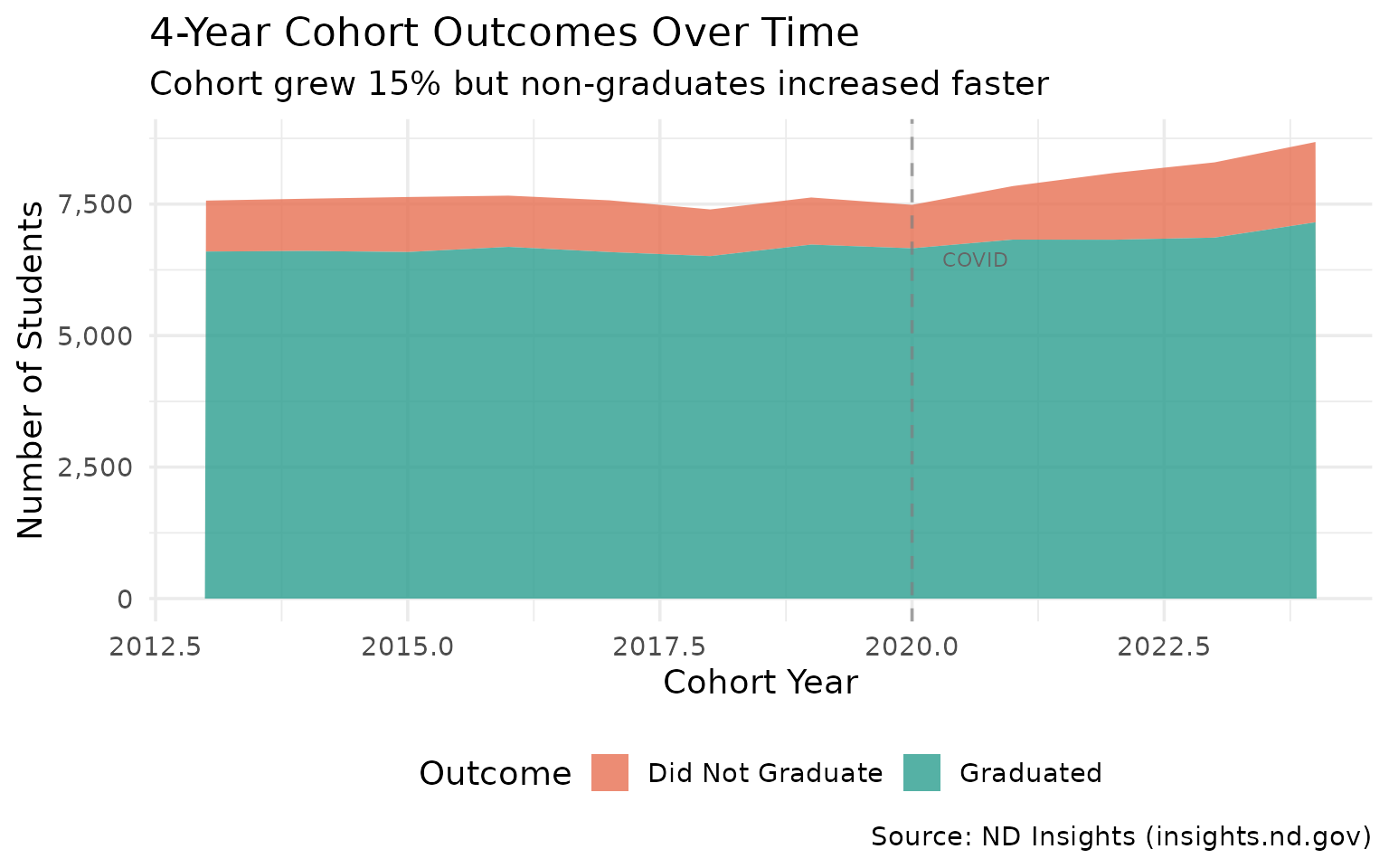
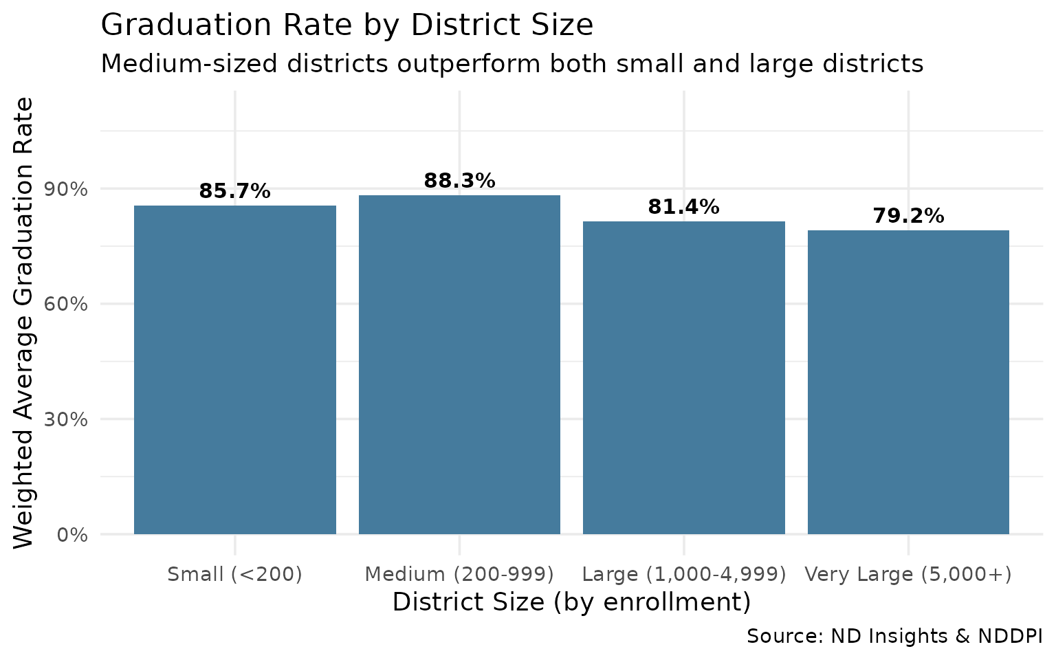
16. Medium-Sized Districts Lead in Graduation Rates
Mid-size districts (200-999 students) outperform both small rural and large urban districts.
# Join enrollment to graduation data
# Note: enrollment uses CC-DDD format, graduation uses CCDDD format
district_size <- enr_2024 %>%
  filter(is_district, subgroup == "total_enrollment", grade_level == "TOTAL") %>%
  mutate(district_id_clean = gsub("-", "", district_id)) %>%
  select(district_id_clean, enrollment = n_students)

grad_with_size <- grad_2024 %>%
  filter(is_district, subgroup == "all", cohort_count >= 10) %>%
  mutate(district_id_clean = district_id) %>%
  left_join(district_size, by = "district_id_clean") %>%
  mutate(size_category = case_when(
    enrollment < 200 ~ "Small (<200)",
    enrollment < 1000 ~ "Medium (200-999)",
    enrollment < 5000 ~ "Large (1,000-4,999)",
    TRUE ~ "Very Large (5,000+)"
  )) %>%
  filter(!is.na(size_category))

size_summary <- grad_with_size %>%
  group_by(size_category) %>%
  summarize(
    n_districts = n(),
    avg_grad_rate = weighted.mean(grad_rate, cohort_count, na.rm = TRUE),
    total_cohort = sum(cohort_count, na.rm = TRUE),
    .groups = "drop"
  ) %>%
  mutate(size_category = factor(size_category,
                                levels = c("Small (<200)", "Medium (200-999)",
                                          "Large (1,000-4,999)", "Very Large (5,000+)")))

stopifnot(nrow(size_summary) > 0)
size_summary
#> # A tibble: 4 × 4
#>   size_category       n_districts avg_grad_rate total_cohort
#>   <fct>                     <int>         <dbl>        <int>
#> 1 Large (1,000-4,999)           8         0.814         1408
#> 2 Medium (200-999)             79         0.883         2302
#> 3 Small (<200)                 29         0.857          418
#> 4 Very Large (5,000+)           6         0.792         4414
ggplot(size_summary, aes(x = size_category, y = avg_grad_rate)) +
  geom_col(fill = "#457B9D") +
  geom_text(aes(label = paste0(round(avg_grad_rate * 100, 1), "%")),
            vjust = -0.5, size = 4, fontface = "bold") +
  scale_y_continuous(labels = scales::percent, limits = c(0, 1.1)) +
  labs(
    title = "Graduation Rate by District Size",
    subtitle = "Medium-sized districts outperform both small and large districts",
    x = "District Size (by enrollment)",
    y = "Weighted Average Graduation Rate",
    caption = "Source: ND Insights & NDDPI"
  )
Learn More
These insights just scratch the surface. Use
ndschooldata to explore:
- Individual district trends over time
- Grade-level patterns within districts
- Regional comparisons across the state
# Get started
library(ndschooldata)

# Fetch all available years
enr_all <- fetch_enr_multi(get_available_years()$min_year:get_available_years()$max_year, use_cache = TRUE)

# Explore your district
enr_all %>%
  filter(grepl("Your District", district_name))
Session Info
sessionInfo()
#> R version 4.5.2 (2025-10-31)
#> Platform: x86_64-pc-linux-gnu
#> Running under: Ubuntu 24.04.3 LTS
#>
#> Matrix products: default
#> BLAS:   /usr/lib/x86_64-linux-gnu/openblas-pthread/libblas.so.3
#> LAPACK: /usr/lib/x86_64-linux-gnu/openblas-pthread/libopenblasp-r0.3.26.so;  LAPACK version 3.12.0
#>
#> locale:
#>  [1] LC_CTYPE=C.UTF-8       LC_NUMERIC=C           LC_TIME=C.UTF-8
#>  [4] LC_COLLATE=C.UTF-8     LC_MONETARY=C.UTF-8    LC_MESSAGES=C.UTF-8
#>  [7] LC_PAPER=C.UTF-8       LC_NAME=C              LC_ADDRESS=C
#> [10] LC_TELEPHONE=C         LC_MEASUREMENT=C.UTF-8 LC_IDENTIFICATION=C
#>
#> time zone: UTC
#> tzcode source: system (glibc)
#>
#> attached base packages:
#> [1] stats     graphics  grDevices utils     datasets  methods   base
#>
#> other attached packages:
#> [1] ggplot2_4.0.2      tidyr_1.3.2        dplyr_1.2.0        ndschooldata_0.1.0
#>
#> loaded via a namespace (and not attached):
#>  [1] rappdirs_0.3.4     sass_0.4.10        utf8_1.2.6         generics_0.1.4
#>  [5] stringi_1.8.7      hms_1.1.4          digest_0.6.39      magrittr_2.0.4
#>  [9] evaluate_1.0.5     grid_4.5.2         RColorBrewer_1.1-3 fastmap_1.2.0
#> [13] cellranger_1.1.0   jsonlite_2.0.0     httr_1.4.8         purrr_1.2.1
#> [17] scales_1.4.0       codetools_0.2-20   textshaping_1.0.5  jquerylib_0.1.4
#> [21] cli_3.6.5          crayon_1.5.3       rlang_1.1.7        bit64_4.6.0-1
#> [25] withr_3.0.2        cachem_1.1.0       yaml_2.3.12        parallel_4.5.2
#> [29] tools_4.5.2        tzdb_0.5.0         curl_7.0.0         vctrs_0.7.1
#> [33] R6_2.6.1           lifecycle_1.0.5    stringr_1.6.0      bit_4.6.0
#> [37] fs_1.6.7           vroom_1.7.0        ragg_1.5.1         pkgconfig_2.0.3
#> [41] desc_1.4.3         pkgdown_2.2.0      pillar_1.11.1      bslib_0.10.0
#> [45] gtable_0.3.6       glue_1.8.0         systemfonts_1.3.2  xfun_0.56
#> [49] tibble_3.3.1       tidyselect_1.2.1   knitr_1.51         farver_2.1.2
#> [53] htmltools_0.5.9    rmarkdown_2.30     labeling_0.4.3     readr_2.2.0
#> [57] compiler_4.5.2     S7_0.2.1           readxl_1.4.5