Fetch and analyze North Dakota school enrollment and graduation data from the North Dakota Department of Public Instruction in R or Python.
Part of the njschooldata family.
Full documentation — all 16 stories with interactive charts, getting-started guide, and complete function reference.
Highlights
library(ndschooldata)
library(dplyr)
library(tidyr)
library(ggplot2)
theme_set(theme_minimal(base_size = 14))

enr <- tryCatch(
  fetch_enr_multi(2008:2024, use_cache = TRUE),
  error = function(e) {
    warning("Failed to fetch enrollment data: ", e$message)
    stop(e)
  }
)
1. Graduation rates dropped 7 points from their peak
The statewide graduation rate peaked at 89% in 2020 and has declined to 82% in four years.
grad_multi <- tryCatch(
  fetch_graduation_multi(2013:2024, use_cache = TRUE),
  error = function(e) {
    warning("Failed to fetch graduation data: ", e$message)
    stop(e)
  }
)

grad_trend <- grad_multi %>%
  filter(is_state, subgroup == "all") %>%
  select(end_year, grad_rate, cohort_count, graduate_count)

stopifnot(nrow(grad_trend) > 0)
grad_trend
#>    end_year grad_rate cohort_count graduate_count
#> 1      2013     0.872         7567           6598
#> 2      2014     0.869         7603           6609
#> 3      2015     0.863         7635           6589
#> 4      2016     0.873         7661           6687
#> 5      2017     0.870         7572           6588
#> 6      2018     0.880         7399           6512
#> 7      2019     0.883         7626           6730
#> 8      2020     0.890         7486           6660
#> 9      2021     0.870         7843           6825
#> 10     2022     0.843         8092           6823
#> 11     2023     0.827         8294           6863
#> 12     2024     0.824         8681           7154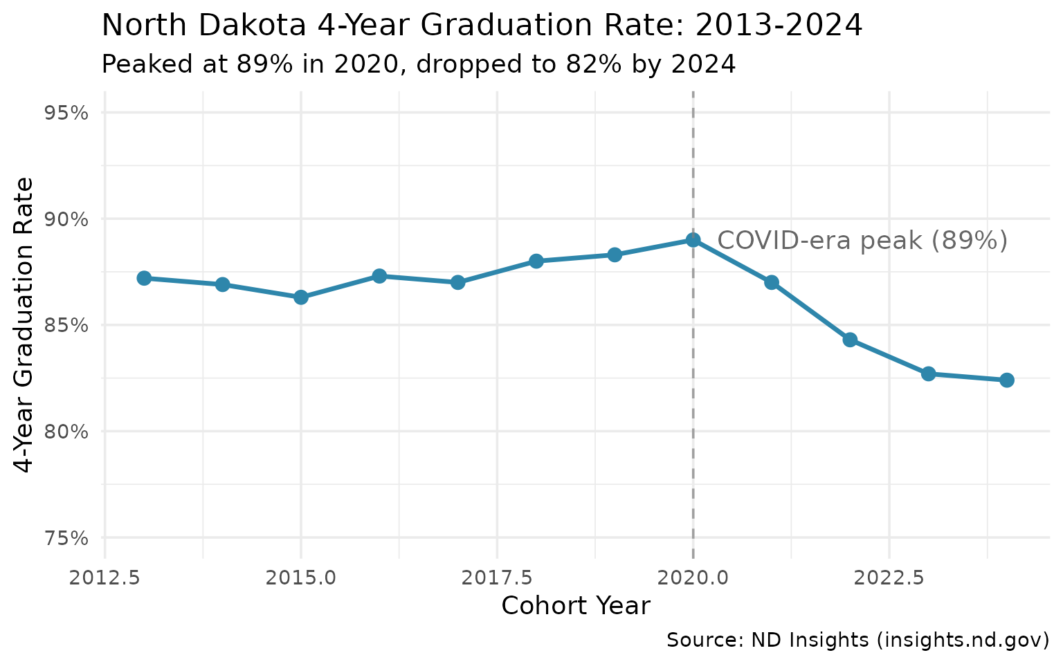
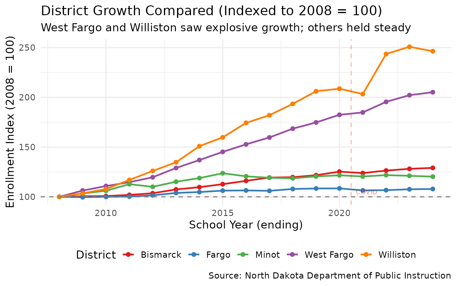
2. West Fargo doubled in size since 2008
The Fargo suburb is one of the fastest-growing districts in the country.
growth_districts <- enr %>%
  filter(is_district, subgroup == "total_enrollment", grade_level == "TOTAL",
         grepl("West Fargo|Fargo|Bismarck|Williston|Minot", district_name)) %>%
  mutate(district_name = trimws(gsub(" Public Schools| School District| Basin| [0-9]+$", "", district_name))) %>%
  filter(district_name %in% c("Fargo", "West Fargo", "Bismarck", "Williston", "Minot"))

stopifnot(nrow(growth_districts) > 0)

# Normalize to 2008 baseline
growth_indexed <- growth_districts %>%
  group_by(district_name) %>%
  mutate(baseline = n_students[end_year == min(end_year)],
         index = n_students / baseline * 100) %>%
  ungroup()

growth_indexed %>%
  filter(end_year %in% c(2008, 2024)) %>%
  select(district_name, end_year, n_students, index)
#>   district_name end_year n_students    index
#> 1      Bismarck     2008      10638 100.0000
#> 2         Fargo     2008      10493 100.0000
#> 3    West Fargo     2008       6179 100.0000
#> 4         Minot     2008       6243 100.0000
#> 5     Williston     2008       2110 100.0000
#> 6      Bismarck     2024      13732 129.0844
#> 7         Fargo     2024      11319 107.8719
#> 8    West Fargo     2024      12676 205.1465
#> 9         Minot     2024       7510 120.2947
#> 10    Williston     2024       5198 246.3507
+105% growth since 2008. West Fargo went from 6,179 to 12,676 students.
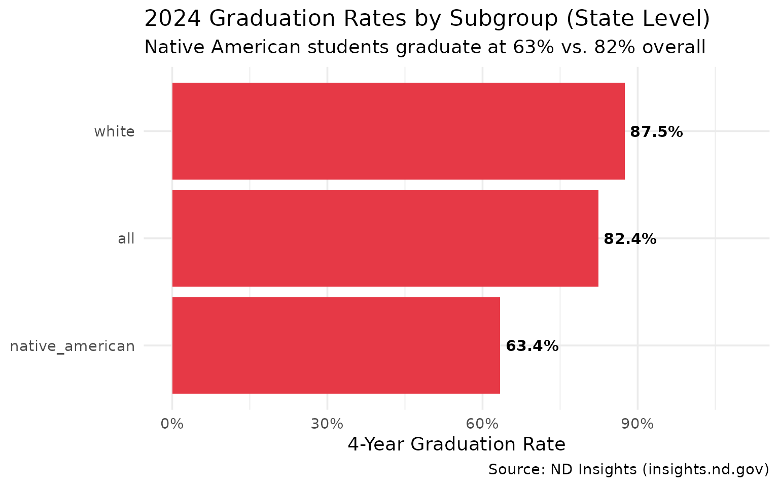
3. Native American graduation rates lag state average
Native American students face a 19-point graduation gap compared to the state average.
grad_2024 <- tryCatch(
  fetch_graduation(2024, use_cache = TRUE),
  error = function(e) {
    warning("Failed to fetch 2024 graduation data: ", e$message)
    stop(e)
  }
)

# Compare subgroups at state level
grad_subgroups <- grad_2024 %>%
  filter(is_state, subgroup %in% c("all", "native_american", "white", "low_income")) %>%
  select(subgroup, grad_rate, cohort_count, graduate_count) %>%
  arrange(desc(grad_rate))

stopifnot(nrow(grad_subgroups) > 0)
grad_subgroups
#>          subgroup grad_rate cohort_count graduate_count
#> 1           white     0.875         6420           5620
#> 2             all     0.824         8681           7154
#> 3      low_income     0.676         2302           1556
#> 4 native_american     0.634          939            595
Native American students graduate at 63% compared to 82% overall. A 19-point gap that demands attention.
Data Taxonomy
| Category | Years | Function | Details |
|---|---|---|---|
| Enrollment | 2008-2024 |
fetch_enr() / fetch_enr_multi()
|
State, district. Grade level (K-12) |
| Assessments | — | — | Not yet available |
| Graduation | 2013-2024 |
fetch_graduation() / fetch_graduation_multi()
|
State, district, school. Race, gender, FRPL, SpEd, LEP |
| Directory | 2014-2024 |
fetch_directory() / fetch_district_directory()
|
School and district. Names, contacts, addresses, coordinates |
| Per-Pupil Spending | — | — | Not yet available |
| Accountability | — | — | Not yet available |
| Chronic Absence | — | — | Not yet available |
| EL Progress | — | — | Not yet available |
| Special Ed | — | — | Not yet available |
See DATA-CATEGORY-TAXONOMY.md for what each category covers.
Quick Start
R
# install.packages("remotes")
remotes::install_github("almartin82/ndschooldata")
library(ndschooldata)
library(dplyr)

# Fetch one year
enr_2024 <- fetch_enr(2024, use_cache = TRUE)

# Fetch multiple years
enr_recent <- fetch_enr_multi(2019:2024, use_cache = TRUE)

# State totals
enr_2024 %>%
  filter(is_state, subgroup == "total_enrollment", grade_level == "TOTAL")

# District breakdown
enr_2024 %>%
  filter(is_district, subgroup == "total_enrollment", grade_level == "TOTAL") %>%
  arrange(desc(n_students))

# Check available years
get_available_years()

# Fetch graduation rates
grad_2024 <- fetch_graduation(2024, use_cache = TRUE)

# State graduation rate
grad_2024 %>%
  filter(is_state, subgroup == "all") %>%
  select(grad_rate, cohort_count, graduate_count)

# District graduation rates
grad_2024 %>%
  filter(is_district, subgroup == "all") %>%
  arrange(desc(grad_rate)) %>%
  select(district_name, grad_rate, cohort_count)

# Graduation rate by subgroup (state level)
grad_2024 %>%
  filter(is_state, subgroup %in% c("all", "male", "female", "native_american", "white")) %>%
  select(subgroup, grad_rate, cohort_count)
Python
import pyndschooldata as nd

# Fetch one year
enr_2024 = nd.fetch_enr(2024)

# Fetch multiple years
enr_recent = nd.fetch_enr_multi([2019, 2020, 2021, 2022, 2023, 2024])

# State totals
state_totals = enr_2024[
    (enr_2024['is_state'] == True) &
    (enr_2024['subgroup'] == 'total_enrollment') &
    (enr_2024['grade_level'] == 'TOTAL')
]

# District breakdown
district_totals = enr_2024[
    (enr_2024['is_district'] == True) &
    (enr_2024['subgroup'] == 'total_enrollment') &
    (enr_2024['grade_level'] == 'TOTAL')
].sort_values('n_students', ascending=False)

# Check available years
years = nd.get_available_years()
print(f"Data available from {years['min_year']} to {years['max_year']}")
Explore More
- Full documentation — 16 stories with charts
- Enrollment vignette — 16 stories
- Function reference
Data Notes
Data Sources
- Enrollment: North Dakota DPI (nd.gov/dpi/data)
- Graduation: ND Insights (insights.nd.gov)
Data Availability
| Data Type | Years | Source | Notes |
|---|---|---|---|
| Enrollment | 2008-2024 | NDDPI | District-level enrollment by grade (K-12) |
| Graduation | 2013-2024 | ND Insights | 4-year cohort graduation rates (state, district, school) |
| Directory | 2014-2024 | ND Insights | School and district names, contacts, addresses |
Suppression Rules
- Graduation data: Cohorts with fewer than 10 students are suppressed (marked as * or empty)
- Enrollment data: No suppression in main enrollment files
What’s Included
Enrollment data: - Levels: State, district (~167) - Grade levels: K-12 plus totals - Demographics: Limited (not in main file; available via insights.nd.gov)
Graduation rate data: - Levels: State, district (~167), school (~450) - Years: 2013-2024 (12 years) - Cohort type: 4-year adjusted cohort graduation rate (ACGR) - Subgroups: All, male, female, white, Black, Hispanic, Asian American, Native American, English Learner, IEP, Low Income, and more
Deeper Dive
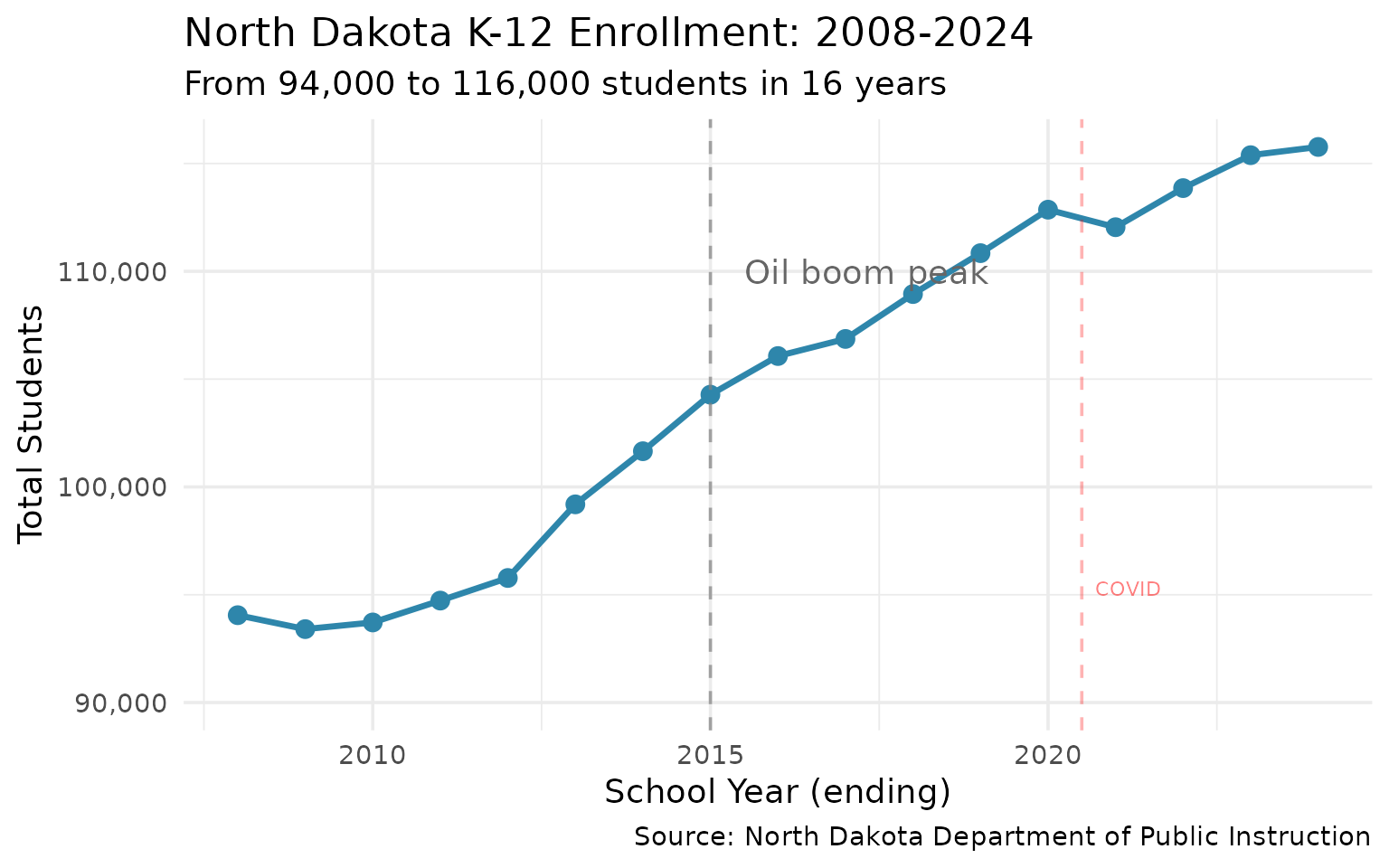
4. The oil boom reshaped North Dakota schools
Enrollment grew 23% from 2008 to 2024 as the Bakken brought families to the state.
statewide <- enr %>%
  filter(is_state, subgroup == "total_enrollment", grade_level == "TOTAL") %>%
  select(end_year, n_students)

stopifnot(nrow(statewide) > 0)
statewide
#>    end_year n_students
#> 1      2008      94052
#> 2      2009      93406
#> 3      2010      93715
#> 4      2011      94729
#> 5      2012      95778
#> ...
#> 17     2024     115767
From 94,000 to 116,000 students in 16 years. The boom changed everything.
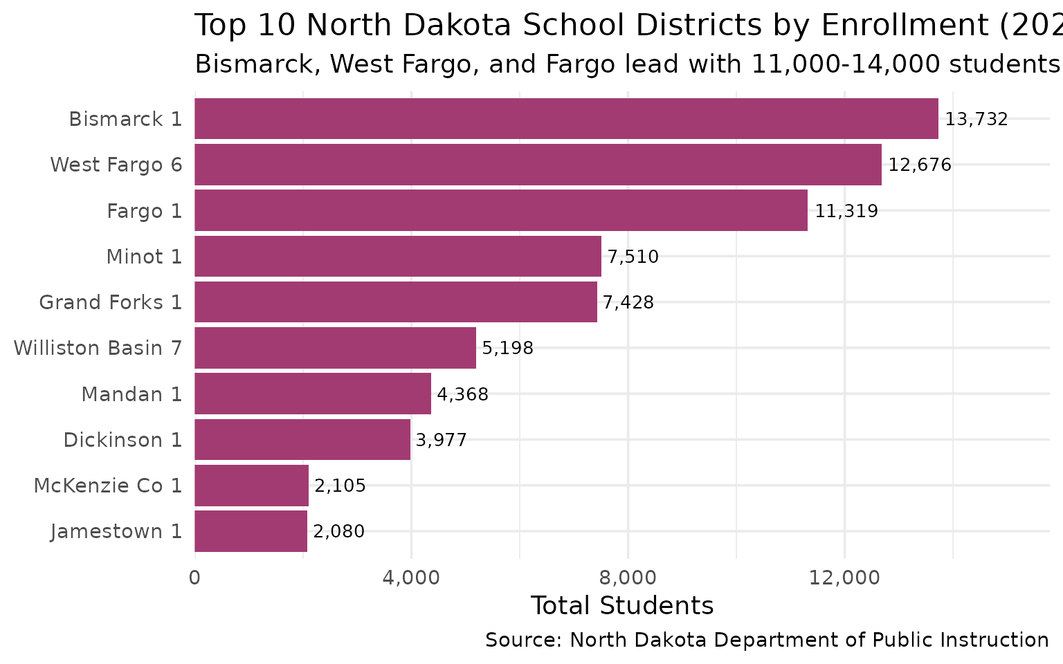
5. Bismarck leads the state in enrollment
The capital city edges out West Fargo and Fargo as the state’s largest district.
enr_2024 <- tryCatch(
  fetch_enr(2024, use_cache = TRUE),
  error = function(e) {
    warning("Failed to fetch 2024 enrollment data: ", e$message)
    stop(e)
  }
)

top_districts <- enr_2024 %>%
  filter(is_district, subgroup == "total_enrollment", grade_level == "TOTAL") %>%
  arrange(desc(n_students)) %>%
  head(10) %>%
  select(district_name, n_students) %>%
  mutate(district_name = gsub(" Public Schools| School District", "", district_name))

stopifnot(nrow(top_districts) > 0)
top_districts
#>      district_name n_students
#> 1       Bismarck 1      13732
#> 2     West Fargo 6      12676
#> 3          Fargo 1      11319
#> 4          Minot 1       7510
#> 5    Grand Forks 1       7428
#> 6 Williston Basin 7      5198
#> 7         Mandan 1       4368
#> 8      Dickinson 1       3977
#> 9    McKenzie Co 1       2105
#> 10     Jamestown 1       2080
Bismarck: 13,732 students. The capital city leads the state, with West Fargo close behind at 12,676.
6. Kindergarten enrollment dropped 10% from its peak
The enrollment wave from the oil boom is aging out. Kindergarten peaked at 9,620 in 2020 and fell to 8,636 by 2024.
grade_levels <- enr %>%
  filter(is_state, subgroup == "total_enrollment") %>%
  mutate(level = case_when(
    grade_level %in% c("K", "01", "02", "03", "04", "05") ~ "Elementary (K-5)",
    grade_level %in% c("06", "07", "08") ~ "Middle (6-8)",
    grade_level %in% c("09", "10", "11", "12") ~ "High School (9-12)",
    TRUE ~ NA_character_
  )) %>%
  filter(!is.na(level)) %>%
  group_by(end_year, level) %>%
  summarize(total = sum(n_students, na.rm = TRUE), .groups = "drop")

stopifnot(nrow(grade_levels) > 0)
grade_levels %>% filter(end_year %in% c(2008, 2019, 2024)) %>% arrange(end_year, level)
#>   end_year              level total
#> 1     2008   Elementary (K-5) 40768
#> 2     2008 High School (9-12) 31492
#> 3     2008       Middle (6-8) 21792
#> 4     2019   Elementary (K-5) 53721
#> 5     2019 High School (9-12) 31430
#> 6     2019       Middle (6-8) 25691
#> 7     2024   Elementary (K-5) 54642
#> 8     2024 High School (9-12) 34556
#> 9     2024       Middle (6-8) 26569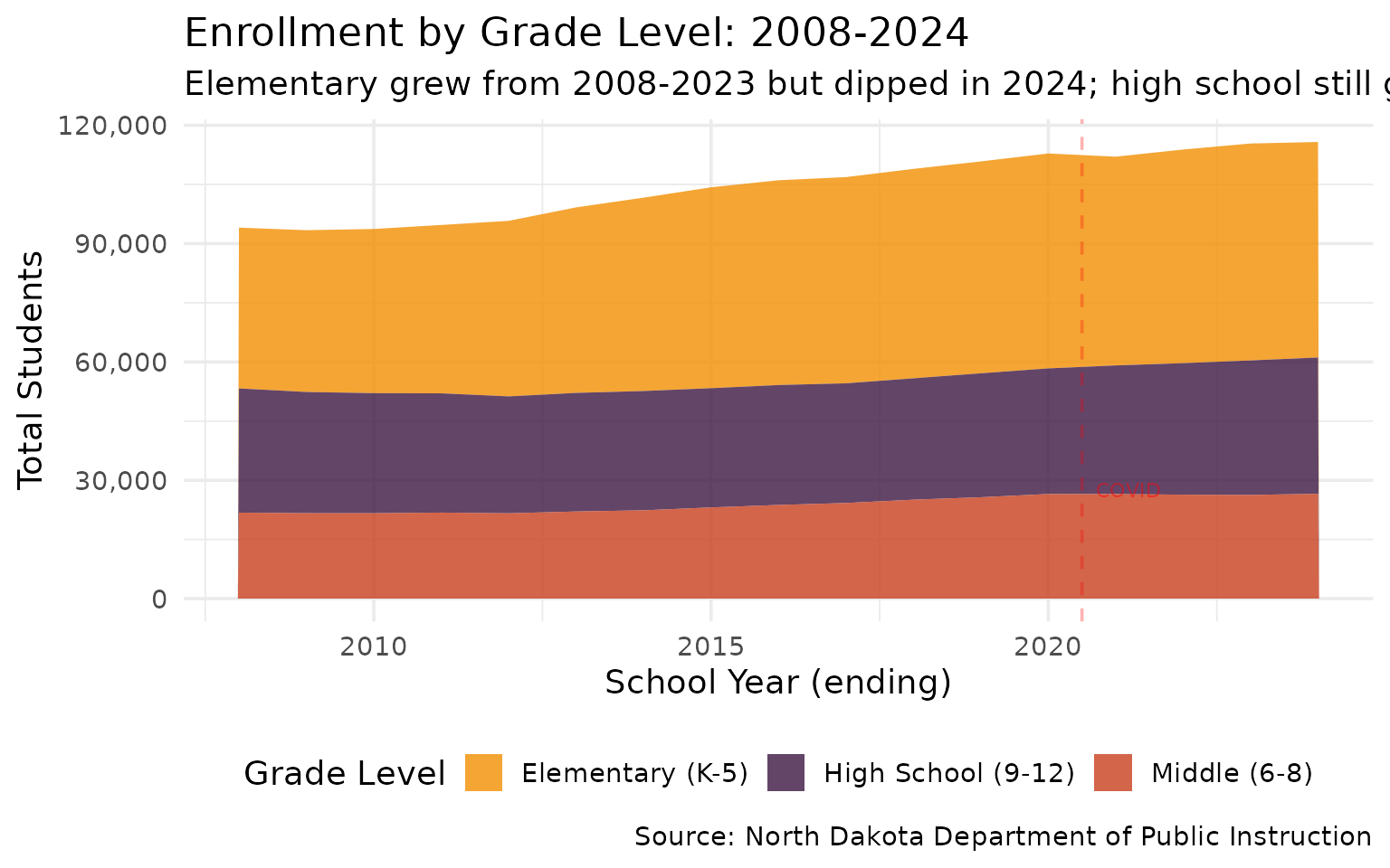
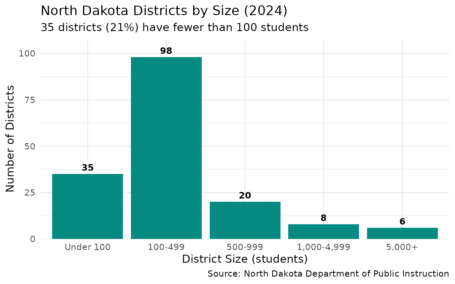
7. 35 districts have under 100 students
Tiny rural schools define the North Dakota landscape.
size_dist <- enr_2024 %>%
  filter(is_district, subgroup == "total_enrollment", grade_level == "TOTAL") %>%
  mutate(size_category = case_when(
    n_students < 100 ~ "Under 100",
    n_students < 500 ~ "100-499",
    n_students < 1000 ~ "500-999",
    n_students < 5000 ~ "1,000-4,999",
    TRUE ~ "5,000+"
  )) %>%
  mutate(size_category = factor(size_category,
                                levels = c("Under 100", "100-499", "500-999",
                                          "1,000-4,999", "5,000+"))) %>%
  count(size_category)

stopifnot(nrow(size_dist) > 0)
size_dist
#>   size_category  n
#> 1     Under 100 35
#> 2       100-499 98
#> 3       500-999 20
#> 4   1,000-4,999  8
#> 5        5,000+  6
35 districts with fewer than 100 students. That’s 21% of all 167 districts.
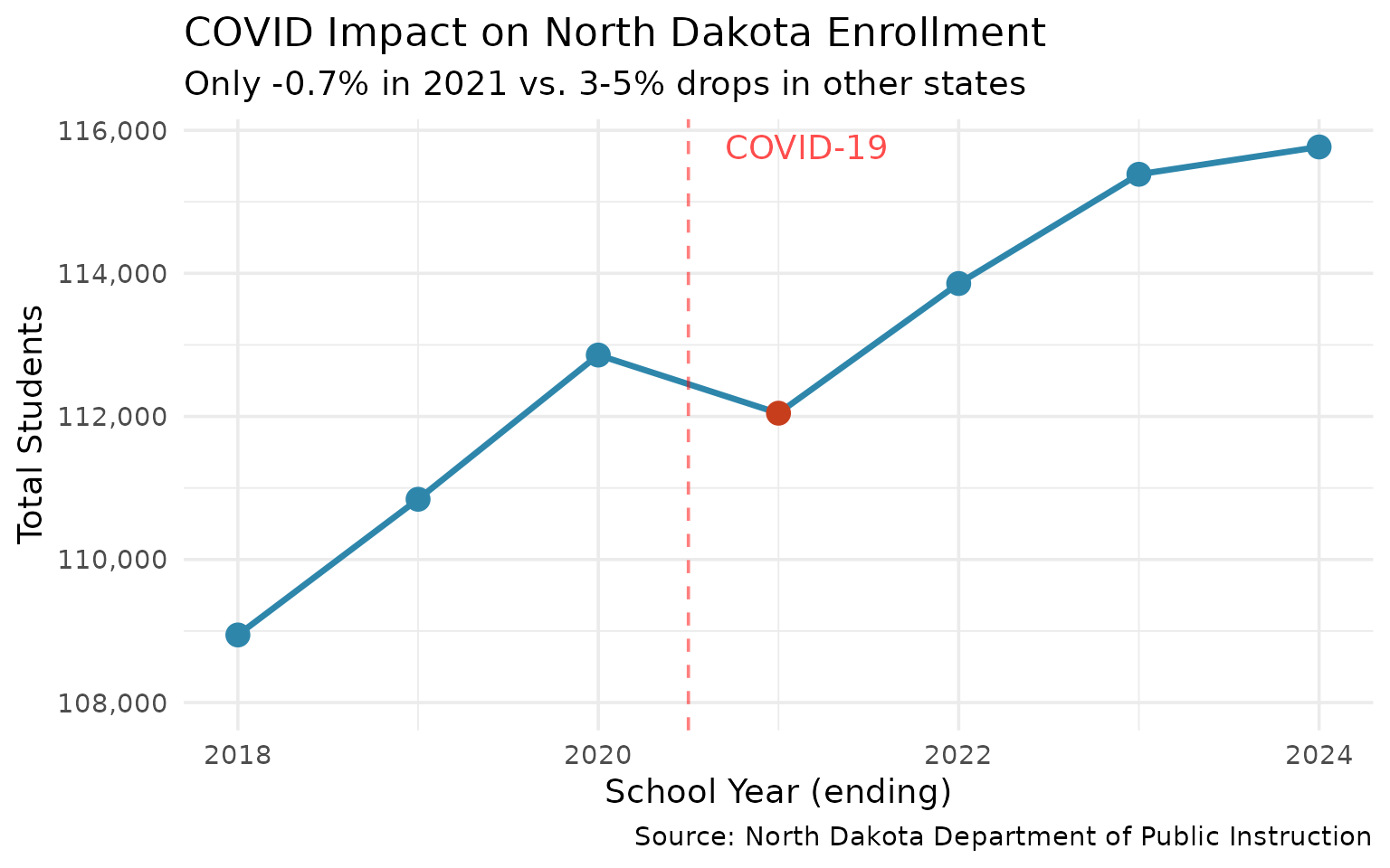
8. COVID barely dented North Dakota enrollment (-0.7%)
Unlike other states, ND saw only a small pandemic drop.
covid_years <- enr %>%
  filter(is_state, subgroup == "total_enrollment", grade_level == "TOTAL",
         end_year %in% 2018:2024) %>%
  select(end_year, n_students) %>%
  mutate(change = n_students - lag(n_students),
         pct_change = round(change / lag(n_students) * 100, 1))

stopifnot(nrow(covid_years) > 0)
covid_years
#>   end_year n_students change pct_change
#> 1     2018     108945     NA         NA
#> 2     2019     110842   1897        1.7
#> 3     2020     112858   2016        1.8
#> 4     2021     112045   -813       -0.7
#> 5     2022     113858   1813        1.6
#> 6     2023     115385   1527        1.3
#> 7     2024     115767    382        0.3
Only -0.7% in 2021. Most states lost 3-5%. Rural schools stayed open.
9. Oil counties vs. traditional farming areas
The Bakken oil formation transformed Williams and McKenzie counties while agricultural areas stayed flat.
oil_districts <- enr %>%
  filter(is_district, subgroup == "total_enrollment", grade_level == "TOTAL",
         grepl("Williston|Watford|Tioga|Alexander|Dickinson|Mandan", district_name)) %>%
  mutate(region = case_when(
    grepl("Williston|Watford|Tioga|Alexander", district_name) ~ "Oil Counties",
    TRUE ~ "Traditional"
  )) %>%
  group_by(end_year, region) %>%
  summarize(total = sum(n_students, na.rm = TRUE), .groups = "drop")

stopifnot(nrow(oil_districts) > 0)
oil_districts %>% filter(end_year %in% c(2008, 2015, 2024))
#>   end_year       region total
#> 1     2008 Oil Counties  2412
#> 2     2008  Traditional  5629
#> 3     2015 Oil Counties  4035
#> 4     2015  Traditional  6879
#> 5     2024 Oil Counties  6052
#> 6     2024  Traditional  8345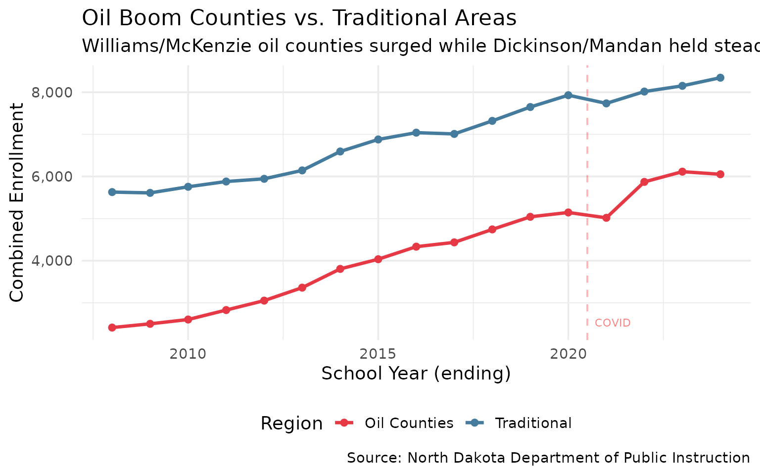
10. Bismarck: steady growth as state capital
While West Fargo doubled in size, Bismarck’s enrollment has grown steadily without the volatility.
bismarck_growth <- enr %>%
  filter(is_district, subgroup == "total_enrollment", grade_level == "TOTAL",
         grepl("Bismarck|Fargo|West Fargo", district_name)) %>%
  mutate(district_name = trimws(gsub(" Public Schools| School District| [0-9]+$", "", district_name))) %>%
  filter(district_name %in% c("Bismarck", "Fargo", "West Fargo")) %>%
  group_by(district_name) %>%
  mutate(yoy_change = (n_students - lag(n_students)) / lag(n_students) * 100) %>%
  ungroup() %>%
  filter(!is.na(yoy_change))

stopifnot(nrow(bismarck_growth) > 0)
bismarck_growth %>%
  group_by(district_name) %>%
  summarize(avg_yoy = round(mean(yoy_change, na.rm = TRUE), 2),
            max_yoy = round(max(yoy_change, na.rm = TRUE), 2),
            min_yoy = round(min(yoy_change, na.rm = TRUE), 2))
#>   district_name avg_yoy max_yoy min_yoy
#> 1      Bismarck    1.62    3.72   -1.16
#> 2         Fargo    0.48    2.39   -1.87
#> 3    West Fargo    4.61    7.78    1.33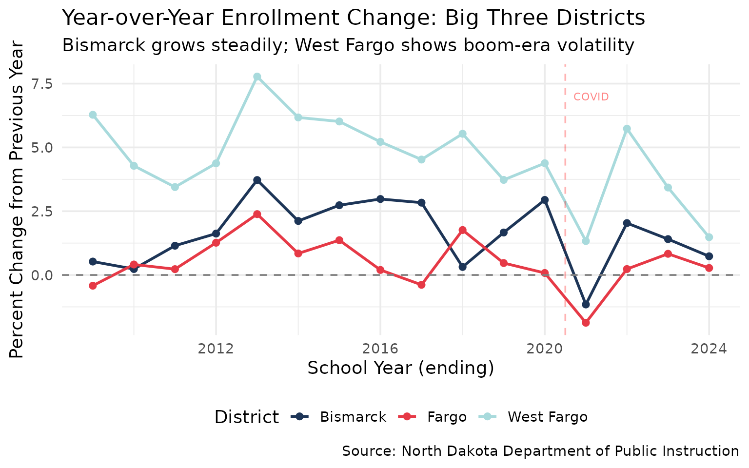
11. Kindergarten as a leading indicator
Kindergarten enrollment predicts total enrollment 12 years later. The recent K decline signals future challenges.
k_vs_total <- enr %>%
  filter(is_state, subgroup == "total_enrollment") %>%
  filter(grade_level %in% c("K", "TOTAL")) %>%
  select(end_year, grade_level, n_students) %>%
  pivot_wider(names_from = grade_level, values_from = n_students) %>%
  rename(kindergarten = K, total = TOTAL) %>%
  mutate(k_pct = kindergarten / total * 100)

stopifnot(nrow(k_vs_total) > 0)
k_vs_total %>% select(end_year, kindergarten, k_pct)
#>    end_year kindergarten    k_pct
#> 1      2008         6729 7.154553
#> 2      2009         7214 7.723273
#> 3      2010         7470 7.970976
#> ...
#> 12     2019         9324 8.411974
#> 13     2020         9620 8.523986
#> 14     2021         8992 8.025347
#> ...
#> 17     2024         8636 7.459812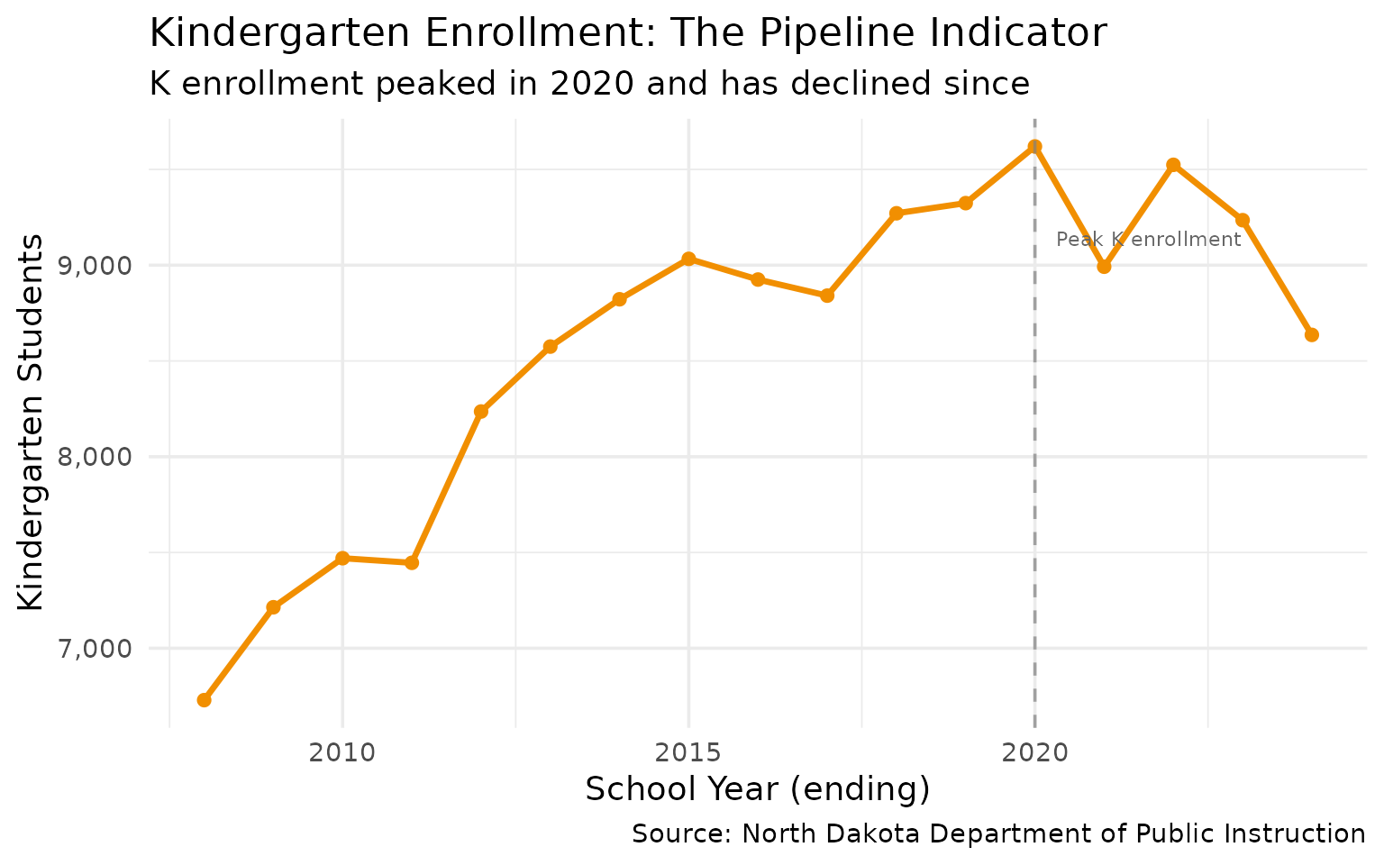
12. Grand Forks: holding steady while others surge
Grand Forks has stabilized while Fargo grew modestly and Minot plateaued after its oil-boom surge.
gf_trend <- enr %>%
  filter(is_district, subgroup == "total_enrollment", grade_level == "TOTAL",
         grepl("Grand Forks|Fargo|Minot", district_name)) %>%
  mutate(district_name = trimws(gsub(" Public Schools| School District| [0-9]+$", "", district_name))) %>%
  filter(district_name %in% c("Grand Forks", "Fargo", "Minot")) %>%
  group_by(district_name) %>%
  mutate(indexed = n_students / first(n_students) * 100) %>%
  ungroup()

stopifnot(nrow(gf_trend) > 0)
gf_trend %>% filter(end_year %in% c(2008, 2016, 2024)) %>% select(district_name, end_year, n_students, indexed)
#>   district_name end_year n_students  indexed
#> 1         Fargo     2008      10493 100.0000
#> 2   Grand Forks     2008       7192 100.0000
#> 3         Minot     2008       6243 100.0000
#> 4         Fargo     2016      11167 106.4233
#> 5   Grand Forks     2016       7264 101.0011
#> 6         Minot     2016       7529 120.5991
#> 7         Fargo     2024      11319 107.8719
#> 8   Grand Forks     2024       7428 103.2814
#> 9         Minot     2024       7510 120.2947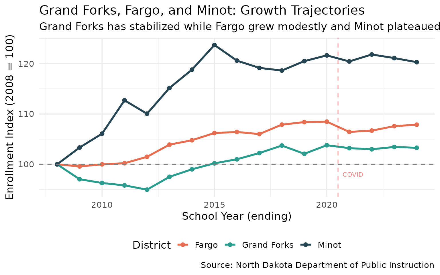
13. The smallest districts are getting smaller
Rural consolidation continues as tiny districts shrink further.
# Track smallest districts over time
small_district_trend <- enr %>%
  filter(is_district, subgroup == "total_enrollment", grade_level == "TOTAL") %>%
  group_by(end_year) %>%
  summarize(
    under_50 = sum(n_students < 50, na.rm = TRUE),
    under_100 = sum(n_students < 100, na.rm = TRUE),
    under_200 = sum(n_students < 200, na.rm = TRUE),
    .groups = "drop"
  ) %>%
  pivot_longer(cols = starts_with("under"), names_to = "category", values_to = "count") %>%
  mutate(category = case_when(
    category == "under_50" ~ "Under 50 students",
    category == "under_100" ~ "Under 100 students",
    category == "under_200" ~ "Under 200 students"
  ))

stopifnot(nrow(small_district_trend) > 0)
small_district_trend %>% filter(end_year %in% c(2008, 2016, 2024)) %>% arrange(end_year, category)
#>   end_year           category count
#> 1     2008 Under 100 students    57
#> 2     2008 Under 200 students   100
#> 3     2008  Under 50 students    33
#> 4     2016 Under 100 students    39
#> 5     2016 Under 200 students    78
#> 6     2016  Under 50 students    20
#> 7     2024 Under 100 students    35
#> 8     2024 Under 200 students    73
#> 9     2024  Under 50 students    13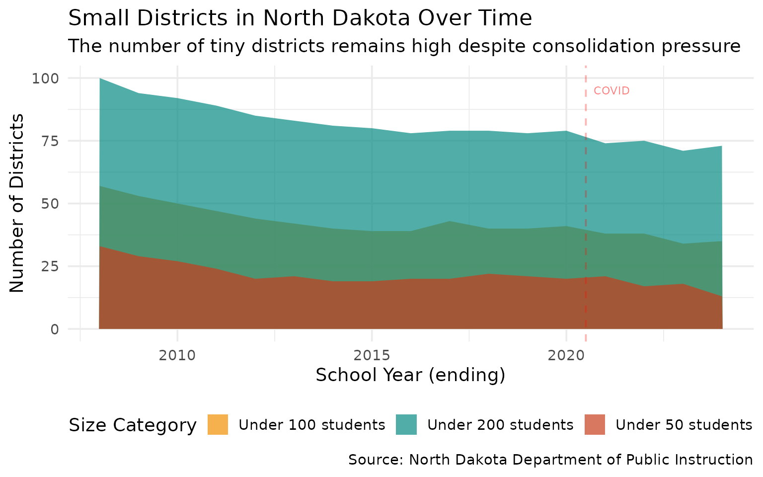
14. McKenzie County leads in graduation rates
Among districts with 100+ student cohorts, the oil-country districts outperform the metro areas.
top_grad_districts <- grad_2024 %>%
  filter(is_district, subgroup == "all", cohort_count >= 100) %>%
  arrange(desc(grad_rate)) %>%
  head(10) %>%
  select(district_name, grad_rate, cohort_count, graduate_count) %>%
  mutate(district_name = gsub(" Public School.*| School District.*", "", district_name))

stopifnot(nrow(top_grad_districts) > 0)
top_grad_districts
#>    district_name grad_rate cohort_count graduate_count
#> 1  McKenzie Co 1     0.858          106             91
#> 2       Mandan 1     0.853          334            285
#> 3     Bismarck 1     0.845         1057            893
#> 4  Grand Forks 1     0.828          599            496
#> 5  Devils Lake 1     0.823          130            107
#> 6    Jamestown 1     0.821          207            170
#> 7        Fargo 1     0.800          949            759
#> 8   West Fargo 6     0.799          884            706
#> 9    Wahpeton 37     0.790          119             94
#> 10   Dickinson 1     0.780          296            231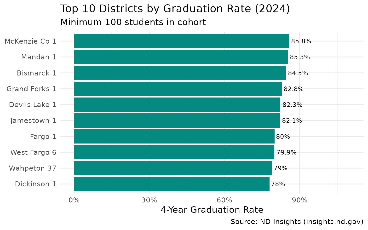
15. Cohort size has grown 15% since 2013
More students are reaching senior year as the oil boom generation ages through.
cohort_trend <- grad_multi %>%
  filter(is_state, subgroup == "all") %>%
  select(end_year, cohort_count, graduate_count) %>%
  mutate(
    non_grad = cohort_count - graduate_count,
    pct_change = round((cohort_count / first(cohort_count) - 1) * 100, 1)
  )

stopifnot(nrow(cohort_trend) > 0)
cohort_trend
#>    end_year cohort_count graduate_count non_grad pct_change
#> 1      2013         7567           6598      969        0.0
#> 2      2014         7603           6609      994        0.5
#> 3      2015         7635           6589     1046        0.9
#> 4      2016         7661           6687      974        1.2
#> 5      2017         7572           6588      984        0.1
#> 6      2018         7399           6512      887       -2.2
#> 7      2019         7626           6730      896        0.8
#> 8      2020         7486           6660      826       -1.1
#> 9      2021         7843           6825     1018        3.6
#> 10     2022         8092           6823     1269        6.9
#> 11     2023         8294           6863     1431        9.6
#> 12     2024         8681           7154     1527       14.7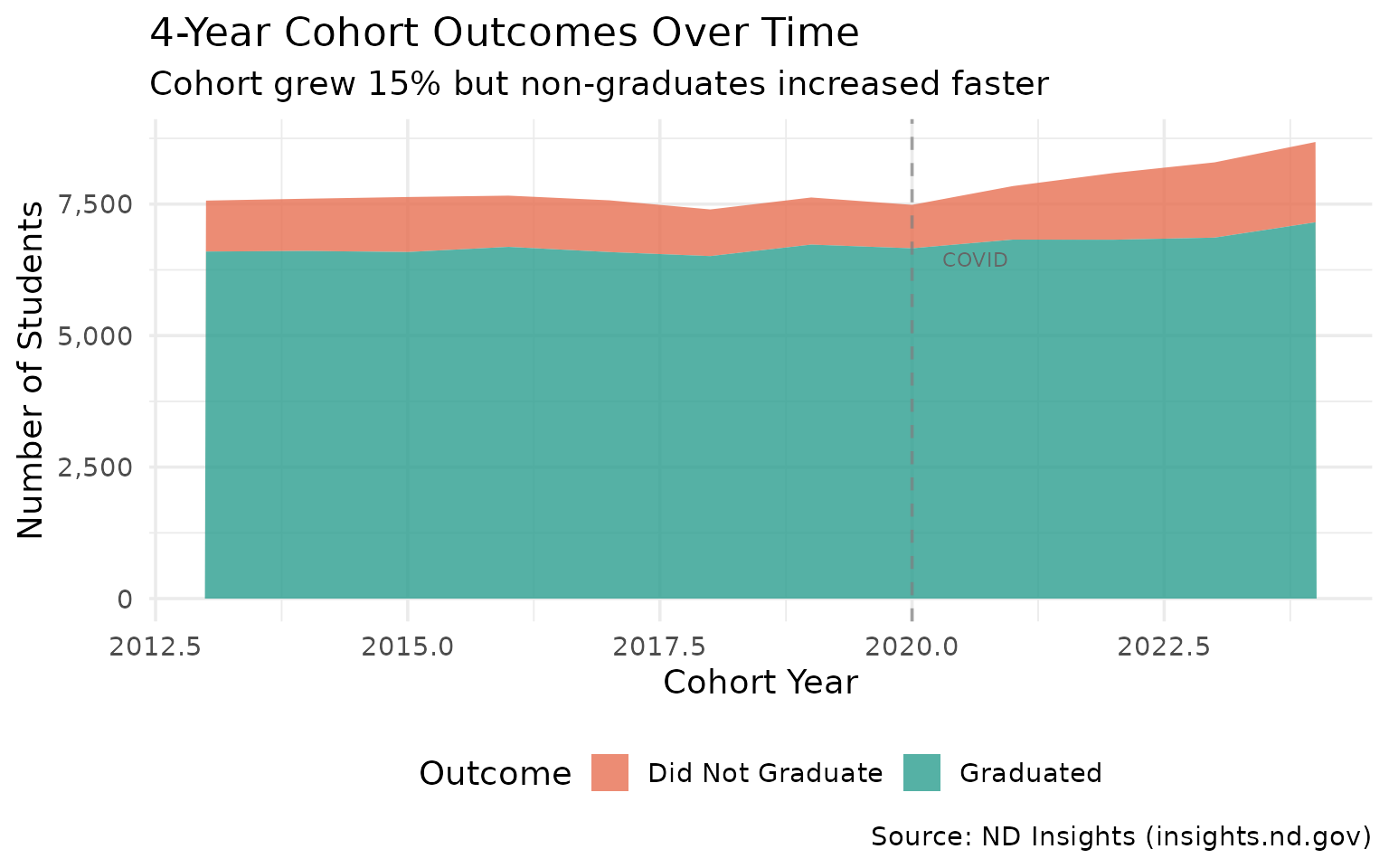
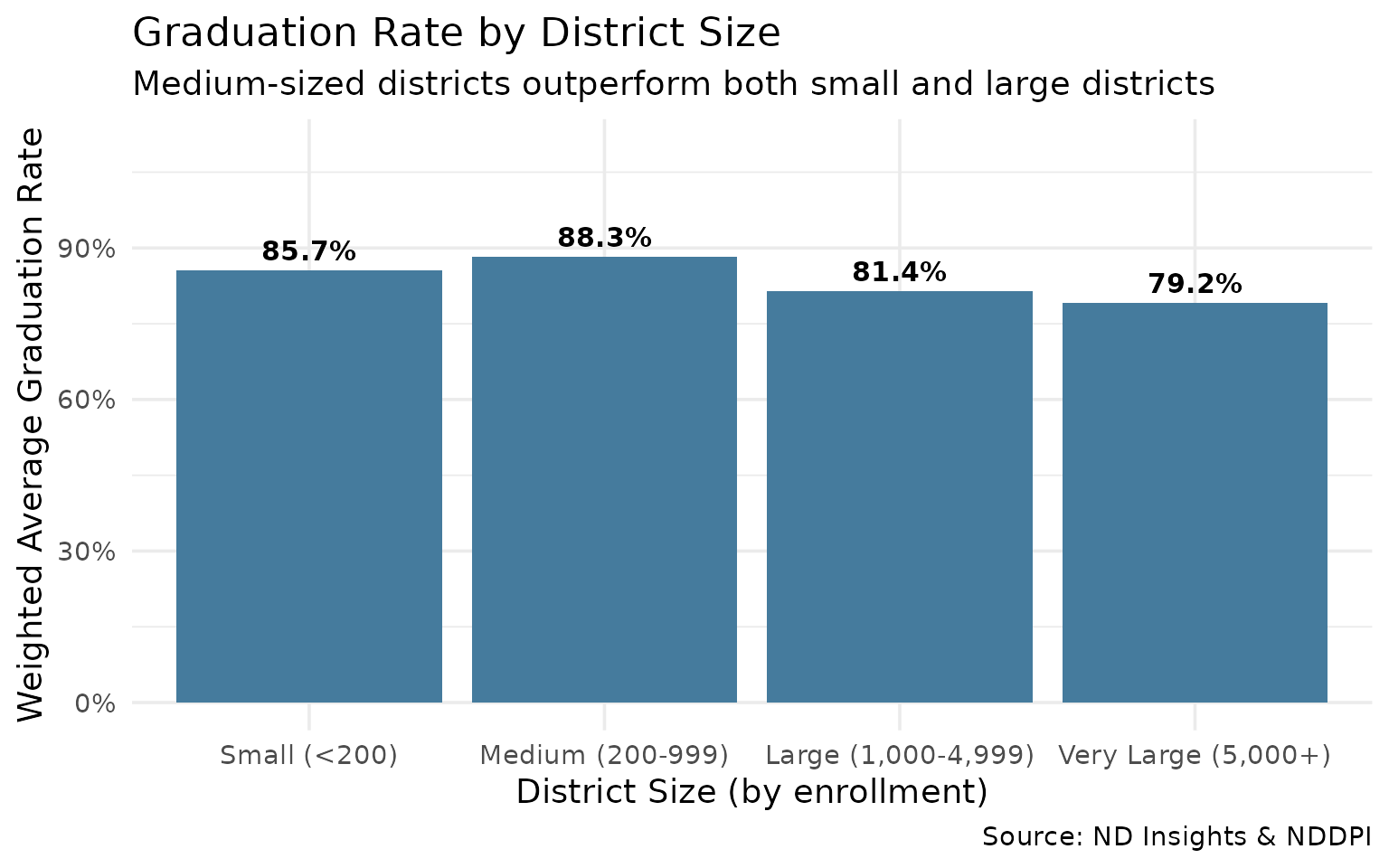
16. Medium-sized districts lead in graduation rates
Mid-size districts (200-999 students) outperform both small rural and large urban districts.
# Join enrollment to graduation data
# Note: enrollment uses CC-DDD format, graduation uses CCDDD format
district_size <- enr_2024 %>%
  filter(is_district, subgroup == "total_enrollment", grade_level == "TOTAL") %>%
  mutate(district_id_clean = gsub("-", "", district_id)) %>%
  select(district_id_clean, enrollment = n_students)

grad_with_size <- grad_2024 %>%
  filter(is_district, subgroup == "all", cohort_count >= 10) %>%
  mutate(district_id_clean = district_id) %>%
  left_join(district_size, by = "district_id_clean") %>%
  mutate(size_category = case_when(
    enrollment < 200 ~ "Small (<200)",
    enrollment < 1000 ~ "Medium (200-999)",
    enrollment < 5000 ~ "Large (1,000-4,999)",
    TRUE ~ "Very Large (5,000+)"
  )) %>%
  filter(!is.na(size_category))

size_summary <- grad_with_size %>%
  group_by(size_category) %>%
  summarize(
    n_districts = n(),
    avg_grad_rate = weighted.mean(grad_rate, cohort_count, na.rm = TRUE),
    total_cohort = sum(cohort_count, na.rm = TRUE),
    .groups = "drop"
  ) %>%
  mutate(size_category = factor(size_category,
                                levels = c("Small (<200)", "Medium (200-999)",
                                          "Large (1,000-4,999)", "Very Large (5,000+)")))

stopifnot(nrow(size_summary) > 0)
size_summary
#>         size_category n_districts avg_grad_rate total_cohort
#> 1       Small (<200)          30     0.8608376          431
#> 2  Medium (200-999)           79     0.8827524         2302
#> 3 Large (1,000-4,999)          8     0.8143729         1408
#> 4 Very Large (5,000+)          6     0.7921319         4414