15 Insights from Nebraska School Enrollment Data
Source:vignettes/enrollment_hooks.Rmd
enrollment_hooks.Rmd
library(neschooldata)
library(dplyr)
library(tidyr)
library(ggplot2)
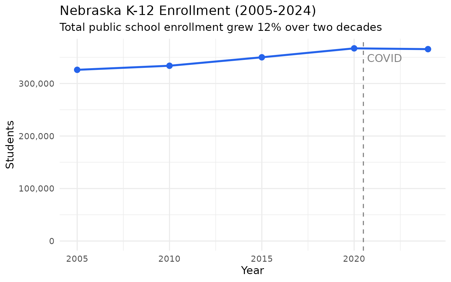
theme_set(theme_minimal(base_size = 14))Nebraska added 39,000 students between 2005 and 2024
Two decades of steady growth – though the pandemic peak in 2020 was actually higher than 2024.
enr <- fetch_enr_multi(c(2005, 2010, 2015, 2020, 2024), use_cache = TRUE)

statewide <- enr %>%
  filter(is_state, subgroup == "total_enrollment", grade_level == "TOTAL") %>%
  select(end_year, n_students)

stopifnot(nrow(statewide) > 0)
statewide
#>   end_year n_students
#> 1     2005     326083
#> 2     2010     333835
#> 3     2015     349925
#> 4     2020     366966
#> 5     2024     365467
ggplot(statewide, aes(x = end_year, y = n_students)) +
  geom_line(color = "#2563eb", linewidth = 1.2) +
  geom_point(color = "#2563eb", size = 3) +
  geom_vline(xintercept = 2020.5, linetype = "dashed", color = "gray50") +
  annotate("text", x = 2020.5, y = max(statewide$n_students) * 0.95,
           label = "COVID", hjust = -0.1, color = "gray50") +
  scale_y_continuous(labels = scales::comma, limits = c(0, NA)) +
  labs(
    title = "Nebraska K-12 Enrollment (2005-2024)",
    subtitle = "Total public school enrollment grew 12% over two decades",
    x = "Year",
    y = "Students"
  )
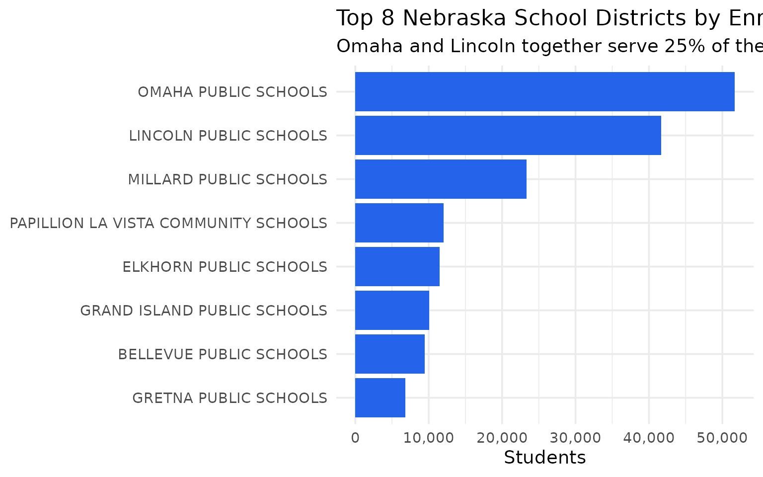
Omaha and Lincoln enroll a quarter of all Nebraska students
The two cities anchor the state’s education system – but they are far from half.
enr_2024 <- fetch_enr(2024, use_cache = TRUE)

top_districts <- enr_2024 %>%
  filter(is_district, subgroup == "total_enrollment", grade_level == "TOTAL") %>%
  arrange(desc(n_students)) %>%
  head(8) %>%
  select(district_name, n_students)

stopifnot(nrow(top_districts) > 0)
top_districts
#>                          district_name n_students
#> 1                 OMAHA PUBLIC SCHOOLS      51693
#> 2               LINCOLN PUBLIC SCHOOLS      41654
#> 3               MILLARD PUBLIC SCHOOLS      23300
#> 4 PAPILLION LA VISTA COMMUNITY SCHOOLS      12039
#> 5               ELKHORN PUBLIC SCHOOLS      11455
#> 6          GRAND ISLAND PUBLIC SCHOOLS      10070
#> 7              BELLEVUE PUBLIC SCHOOLS       9444
#> 8                GRETNA PUBLIC SCHOOLS       6788
top_districts %>%
  mutate(district_name = reorder(district_name, n_students)) %>%
  ggplot(aes(x = n_students, y = district_name)) +
  geom_col(fill = "#2563eb") +
  scale_x_continuous(labels = scales::comma) +
  labs(
    title = "Top 8 Nebraska School Districts by Enrollment (2024)",
    subtitle = "Omaha and Lincoln together serve 25% of the state",
    x = "Students",
    y = NULL
  )
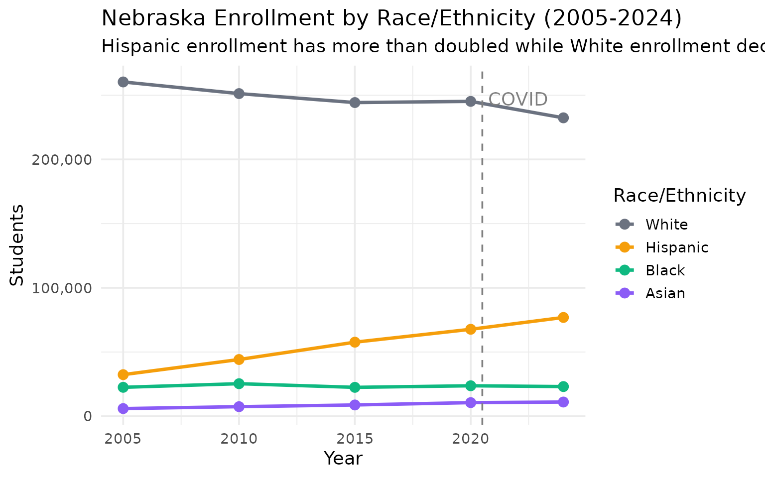
Hispanic enrollment has grown 138% since 2005
Nebraska’s demographic transformation: Hispanic students went from 32,000 to 77,000 in two decades.
demographics <- enr %>%
  filter(is_state, grade_level == "TOTAL",
         subgroup %in% c("white", "hispanic", "black", "asian")) %>%
  select(end_year, subgroup, n_students)

stopifnot(nrow(demographics) > 0)
demographics %>%
  pivot_wider(names_from = subgroup, values_from = n_students)
#> # A tibble: 5 × 5
#>   end_year  white black hispanic asian
#>      <dbl>  <dbl> <dbl>    <dbl> <dbl>
#> 1     2005 260334 22523    32373  5966
#> 2     2010 251265 25340    44171  7445
#> 3     2015 244283 22498    57665  8780
#> 4     2020 245206 23716    67707 10590
#> 5     2024 232394 23100    76933 11061
demographics %>%
  mutate(subgroup = factor(subgroup,
                           levels = c("white", "hispanic", "black", "asian"),
                           labels = c("White", "Hispanic", "Black", "Asian"))) %>%
  ggplot(aes(x = end_year, y = n_students, color = subgroup)) +
  geom_line(linewidth = 1.2) +
  geom_point(size = 3) +
  geom_vline(xintercept = 2020.5, linetype = "dashed", color = "gray50") +
  annotate("text", x = 2020.5, y = max(demographics$n_students) * 0.95,
           label = "COVID", hjust = -0.1, color = "gray50") +
  scale_y_continuous(labels = scales::comma) +
  scale_color_manual(values = c("White" = "#6b7280", "Hispanic" = "#f59e0b",
                                "Black" = "#10b981", "Asian" = "#8b5cf6")) +
  labs(
    title = "Nebraska Enrollment by Race/Ethnicity (2005-2024)",
    subtitle = "Hispanic enrollment has more than doubled while White enrollment declined",
    x = "Year",
    y = "Students",
    color = "Race/Ethnicity"
  )
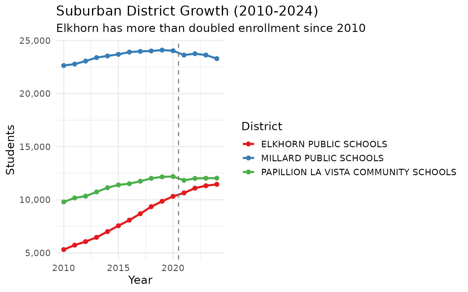
Elkhorn doubled enrollment since 2010
This Omaha suburb grew from 5,300 to 11,500 students in 14 years – the fastest growth in metro Omaha.
enr_multi <- fetch_enr_multi(2010:2024, use_cache = TRUE)

suburban <- enr_multi %>%
  filter(is_district, subgroup == "total_enrollment", grade_level == "TOTAL",
         district_name %in% c("ELKHORN PUBLIC SCHOOLS", "MILLARD PUBLIC SCHOOLS")) %>%
  select(end_year, district_name, n_students)

# Papillion changed names in 2017; combine under one label
papillion <- enr_multi %>%
  filter(is_district, subgroup == "total_enrollment", grade_level == "TOTAL",
         grepl("PAPILLION", district_name)) %>%
  mutate(district_name = "PAPILLION LA VISTA COMMUNITY SCHOOLS") %>%
  select(end_year, district_name, n_students)

suburban <- bind_rows(suburban, papillion)

stopifnot(nrow(suburban) > 0)
suburban %>%
  filter(end_year %in% c(2010, 2015, 2020, 2024)) %>%
  pivot_wider(names_from = end_year, values_from = n_students)
#> # A tibble: 3 × 5
#>   district_name                        `2010` `2015` `2020` `2024`
#>   <chr>                                 <dbl>  <dbl>  <dbl>  <dbl>
#> 1 ELKHORN PUBLIC SCHOOLS                 5306   7553  10322  11455
#> 2 MILLARD PUBLIC SCHOOLS                22647  23702  24038  23300
#> 3 PAPILLION LA VISTA COMMUNITY SCHOOLS   9797  11401  12190  12039
ggplot(suburban, aes(x = end_year, y = n_students, color = district_name)) +
  geom_line(linewidth = 1.2) +
  geom_point(size = 2) +
  geom_vline(xintercept = 2020.5, linetype = "dashed", color = "gray50") +
  scale_y_continuous(labels = scales::comma) +
  scale_color_brewer(palette = "Set1") +
  labs(
    title = "Suburban District Growth (2010-2024)",
    subtitle = "Elkhorn has more than doubled enrollment since 2010",
    x = "Year",
    y = "Students",
    color = "District"
  )
43 fewer tiny districts since 2010
Districts with fewer than 200 students dropped from 198 to 155 – consolidation in action.
regional <- enr_multi %>%
  filter(is_district, subgroup == "total_enrollment", grade_level == "TOTAL") %>%
  filter(end_year %in% c(2010, 2024)) %>%
  mutate(size = case_when(
    n_students >= 10000 ~ "Large (10,000+)",
    n_students >= 1000 ~ "Medium (1,000-9,999)",
    n_students >= 200 ~ "Small (200-999)",
    TRUE ~ "Tiny (<200)"
  )) %>%
  group_by(end_year, size) %>%
  summarize(n_districts = n(), total_students = sum(n_students), .groups = "drop")

stopifnot(nrow(regional) > 0)
regional %>%
  pivot_wider(names_from = end_year, values_from = c(n_districts, total_students))
#> # A tibble: 4 × 5
#>   size                 n_districts_2010 n_districts_2024 total_students_2010
#>   <chr>                           <int>            <int>               <dbl>
#> 1 Large (10,000+)                     3                6              106250
#> 2 Medium (1,000-9,999)               38               38              113409
#> 3 Small (200-999)                   224              224               95267
#> 4 Tiny (<200)                       198              155               18909
#> # ℹ 1 more variable: total_students_2024 <dbl>
regional %>%
  mutate(size = factor(size, levels = c("Tiny (<200)", "Small (200-999)",
                                         "Medium (1,000-9,999)", "Large (10,000+)"))) %>%
  ggplot(aes(x = size, y = total_students, fill = factor(end_year))) +
  geom_col(position = "dodge") +
  scale_y_continuous(labels = scales::comma) +
  scale_fill_manual(values = c("2010" = "#94a3b8", "2024" = "#2563eb")) +
  labs(
    title = "Enrollment by District Size (2010 vs 2024)",
    subtitle = "Large districts grew while tiny districts disappeared",
    x = "District Size",
    y = "Total Students",
    fill = "Year"
  ) +
  theme(axis.text.x = element_text(angle = 15, hjust = 1))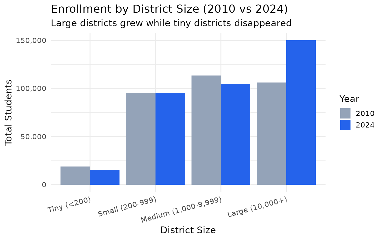
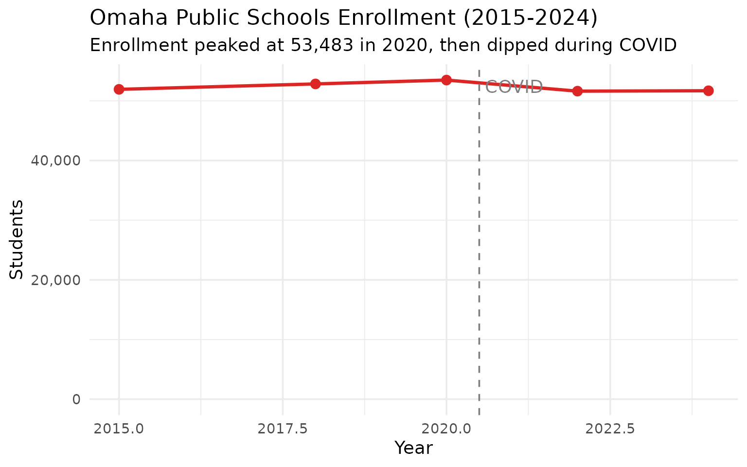
Omaha Public Schools enrollment held steady since 2015
Despite suburban growth, OPS barely changed – from 51,928 in 2015 to 51,693 in 2024.
omaha <- enr_multi %>%
  filter(is_district, subgroup == "total_enrollment", grade_level == "TOTAL",
         district_name == "OMAHA PUBLIC SCHOOLS") %>%
  filter(end_year %in% c(2015, 2018, 2020, 2022, 2024)) %>%
  select(end_year, n_students) %>%
  mutate(change = n_students - lag(n_students))

stopifnot(nrow(omaha) > 0)
omaha
#>   end_year n_students change
#> 1     2015      51928     NA
#> 2     2018      52836    908
#> 3     2020      53483    647
#> 4     2022      51626  -1857
#> 5     2024      51693     67
ggplot(omaha, aes(x = end_year, y = n_students)) +
  geom_line(color = "#dc2626", linewidth = 1.2) +
  geom_point(color = "#dc2626", size = 3) +
  geom_vline(xintercept = 2020.5, linetype = "dashed", color = "gray50") +
  annotate("text", x = 2020.5, y = max(omaha$n_students) * 0.98,
           label = "COVID", hjust = -0.1, color = "gray50") +
  scale_y_continuous(labels = scales::comma, limits = c(0, NA)) +
  labs(
    title = "Omaha Public Schools Enrollment (2015-2024)",
    subtitle = "Enrollment peaked at 53,483 in 2020, then dipped during COVID",
    x = "Year",
    y = "Students"
  )
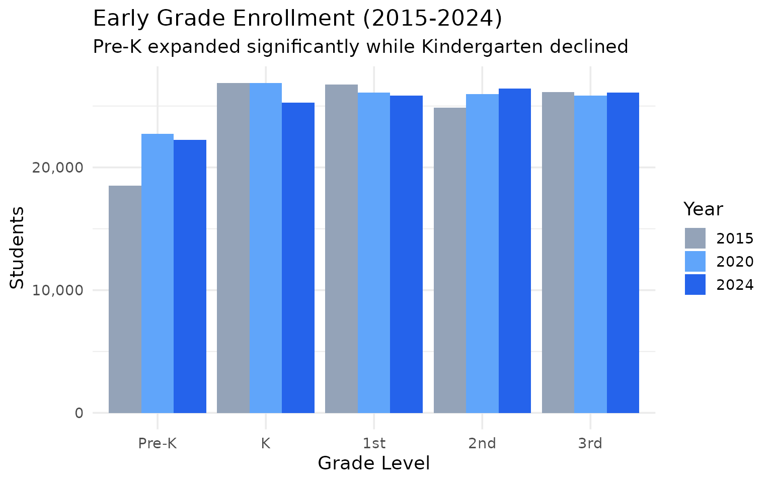
Pre-K grew by 3,768 while Kindergarten shrank by 1,589
Nebraska expanded early childhood access – Pre-K jumped from 18,493 to 22,261 since 2015.
grades <- enr_multi %>%
  filter(is_state, subgroup == "total_enrollment",
         grade_level %in% c("PK", "K", "01", "02", "03")) %>%
  filter(end_year %in% c(2015, 2020, 2024)) %>%
  select(end_year, grade_level, n_students)

stopifnot(nrow(grades) > 0)
grades %>%
  pivot_wider(names_from = end_year, values_from = n_students) %>%
  mutate(change_15_24 = `2024` - `2015`)
#> # A tibble: 5 × 5
#>   grade_level `2015` `2020` `2024` change_15_24
#>   <chr>        <dbl>  <dbl>  <dbl>        <dbl>
#> 1 01           26735  26111  25850         -885
#> 2 02           24853  25991  26415         1562
#> 3 03           26137  25865  26085          -52
#> 4 K            26867  26893  25278        -1589
#> 5 PK           18493  22718  22261         3768
grades %>%
  mutate(grade_level = factor(grade_level,
                              levels = c("PK", "K", "01", "02", "03"),
                              labels = c("Pre-K", "K", "1st", "2nd", "3rd"))) %>%
  ggplot(aes(x = grade_level, y = n_students, fill = factor(end_year))) +
  geom_col(position = "dodge") +
  scale_y_continuous(labels = scales::comma) +
  scale_fill_manual(values = c("2015" = "#94a3b8", "2020" = "#60a5fa", "2024" = "#2563eb")) +
  labs(
    title = "Early Grade Enrollment (2015-2024)",
    subtitle = "Pre-K expanded significantly while Kindergarten declined",
    x = "Grade Level",
    y = "Students",
    fill = "Year"
  )
Grand Island is 61% Hispanic
The meatpacking industry transformed this central Nebraska city into one of the most Hispanic school districts in the Great Plains.
grand_island <- enr_2024 %>%
  filter(grepl("GRAND ISLAND", district_name, ignore.case = TRUE), is_district,
         grade_level == "TOTAL",
         subgroup %in% c("white", "hispanic", "black", "asian")) %>%
  mutate(pct = round(n_students / sum(n_students) * 100, 1)) %>%
  select(subgroup, n_students, pct) %>%
  arrange(desc(pct))

stopifnot(nrow(grand_island) > 0)
grand_island
#>   subgroup n_students  pct
#> 1 hispanic       5922 60.8
#> 2    white       3301 33.9
#> 3    black        444  4.6
#> 4    asian         79  0.8
grand_island %>%
  mutate(subgroup = factor(subgroup,
                           levels = c("hispanic", "white", "black", "asian"),
                           labels = c("Hispanic", "White", "Black", "Asian"))) %>%
  ggplot(aes(x = reorder(subgroup, -pct), y = pct, fill = subgroup)) +
  geom_col() +
  scale_fill_manual(values = c("Hispanic" = "#f59e0b", "White" = "#6b7280",
                               "Black" = "#10b981", "Asian" = "#8b5cf6")) +
  labs(
    title = "Grand Island Public Schools Demographics (2024)",
    subtitle = "61% Hispanic -- meatpacking transformed this community",
    x = NULL,
    y = "Percent of Enrollment"
  ) +
  theme(legend.position = "none")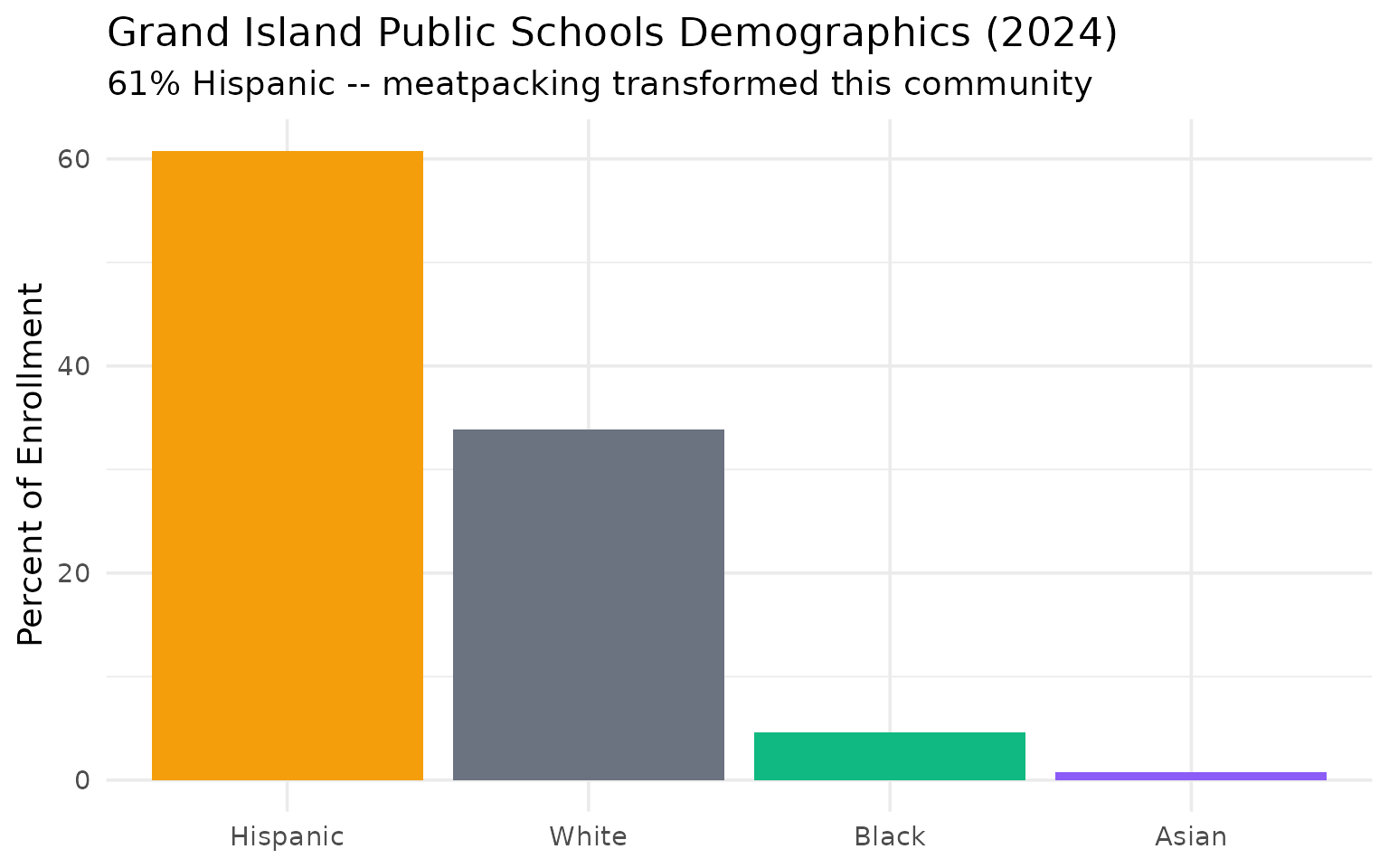
COVID hit Papillion and Omaha hardest, while Elkhorn surged 8%
Between 2019 and 2021, Elkhorn grew while every other major metro district shrank.
covid <- enr_multi %>%
  filter(is_district, subgroup == "total_enrollment", grade_level == "TOTAL",
         district_name %in% c("OMAHA PUBLIC SCHOOLS", "MILLARD PUBLIC SCHOOLS",
                              "ELKHORN PUBLIC SCHOOLS"),
         end_year %in% c(2019, 2021)) %>%
  select(district_name, end_year, n_students)

# Handle Papillion name change
papillion_covid <- enr_multi %>%
  filter(is_district, subgroup == "total_enrollment", grade_level == "TOTAL",
         grepl("PAPILLION", district_name),
         end_year %in% c(2019, 2021)) %>%
  mutate(district_name = "PAPILLION LA VISTA COMMUNITY SCHOOLS") %>%
  select(district_name, end_year, n_students)

covid <- bind_rows(covid, papillion_covid) %>%
  pivot_wider(names_from = end_year, values_from = n_students) %>%
  rename(y2019 = `2019`, y2021 = `2021`) %>%
  mutate(pct_change = round((y2021 - y2019) / y2019 * 100, 1)) %>%
  arrange(pct_change)

stopifnot(nrow(covid) > 0)
covid
#> # A tibble: 4 × 4
#>   district_name                        y2019 y2021 pct_change
#>   <chr>                                <dbl> <dbl>      <dbl>
#> 1 PAPILLION LA VISTA COMMUNITY SCHOOLS 12158 11831       -2.7
#> 2 OMAHA PUBLIC SCHOOLS                 53194 51914       -2.4
#> 3 MILLARD PUBLIC SCHOOLS               24104 23633       -2
#> 4 ELKHORN PUBLIC SCHOOLS                9857 10642        8
covid %>%
  ggplot(aes(x = reorder(district_name, pct_change), y = pct_change,
             fill = pct_change > 0)) +
  geom_col() +
  coord_flip() +
  scale_fill_manual(values = c("TRUE" = "#10b981", "FALSE" = "#dc2626")) +
  labs(
    title = "Enrollment Change During COVID (2019-2021)",
    subtitle = "Elkhorn surged while other metro districts lost students",
    x = NULL,
    y = "Percent Change"
  ) +
  theme(legend.position = "none")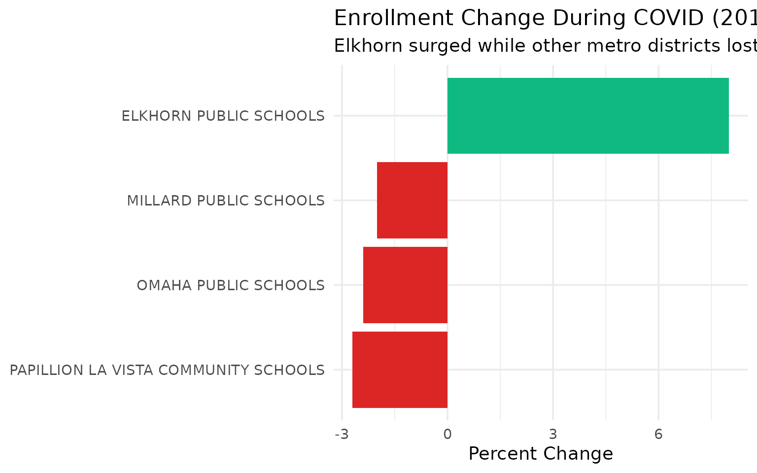
Hispanic students are 21% of the state and growing
Nebraska’s 76,933 Hispanic students are the fastest-growing demographic group.
diversity <- enr_2024 %>%
  filter(is_state, grade_level == "TOTAL") %>%
  filter(subgroup %in% c("total_enrollment", "hispanic", "white", "black", "asian")) %>%
  select(subgroup, n_students) %>%
  mutate(pct = round(n_students / max(n_students) * 100, 1))

stopifnot(nrow(diversity) > 0)
diversity
#>           subgroup n_students   pct
#> 1 total_enrollment     365467 100.0
#> 2            white     232394  63.6
#> 3            black      23100   6.3
#> 4         hispanic      76933  21.1
#> 5            asian      11061   3.0
diversity %>%
  filter(subgroup != "total_enrollment") %>%
  mutate(subgroup = factor(subgroup,
                           levels = c("white", "hispanic", "black", "asian"),
                           labels = c("White", "Hispanic", "Black", "Asian"))) %>%
  ggplot(aes(x = reorder(subgroup, -pct), y = pct, fill = subgroup)) +
  geom_col() +
  scale_fill_manual(values = c("White" = "#6b7280", "Hispanic" = "#f59e0b",
                               "Black" = "#10b981", "Asian" = "#8b5cf6")) +
  labs(
    title = "Nebraska Statewide Demographics (2024)",
    subtitle = "Hispanic students are 21% of enrollment and growing",
    x = NULL,
    y = "Percent of Enrollment"
  ) +
  theme(legend.position = "none")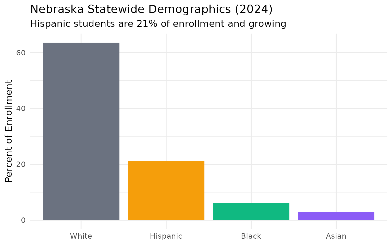
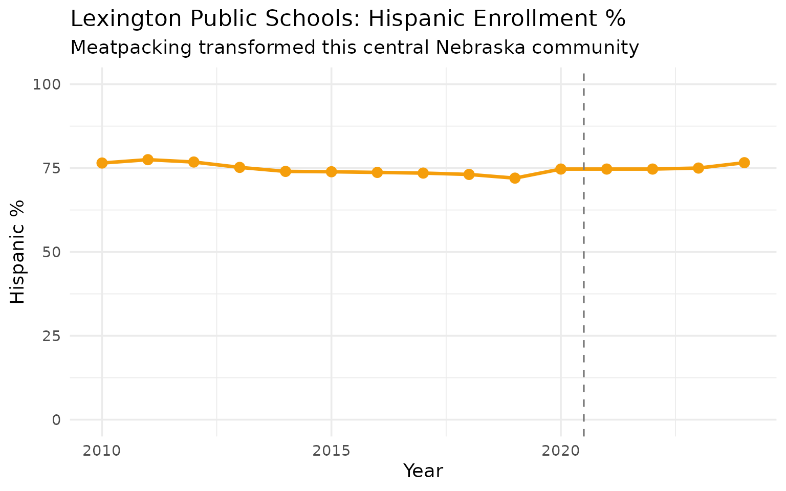
Lexington is 77% Hispanic – a meatpacking transformation
Tyson Foods turned this central Nebraska town from majority-white to majority-Hispanic. The percentage has held steady around 75-77% since 2010.
lexington <- enr_multi %>%
  filter(is_district, grepl("LEXINGTON", district_name, ignore.case = TRUE),
         grade_level == "TOTAL",
         subgroup %in% c("white", "hispanic", "total_enrollment")) %>%
  select(end_year, subgroup, n_students) %>%
  pivot_wider(names_from = subgroup, values_from = n_students) %>%
  mutate(hispanic_pct = round(hispanic / total_enrollment * 100, 1))

stopifnot(nrow(lexington) > 0)
lexington %>%
  filter(end_year %in% c(2010, 2015, 2020, 2024))
#> # A tibble: 4 × 5
#>   end_year total_enrollment white hispanic hispanic_pct
#>      <dbl>            <dbl> <dbl>    <dbl>        <dbl>
#> 1     2010             2804   485     2146         76.5
#> 2     2015             2995   484     2214         73.9
#> 3     2020             3169   444     2368         74.7
#> 4     2024             3229   400     2474         76.6
ggplot(lexington, aes(x = end_year, y = hispanic_pct)) +
  geom_line(color = "#f59e0b", linewidth = 1.2) +
  geom_point(color = "#f59e0b", size = 3) +
  geom_vline(xintercept = 2020.5, linetype = "dashed", color = "gray50") +
  scale_y_continuous(limits = c(0, 100)) +
  labs(
    title = "Lexington Public Schools: Hispanic Enrollment %",
    subtitle = "Meatpacking transformed this central Nebraska community",
    x = "Year",
    y = "Hispanic %"
  )
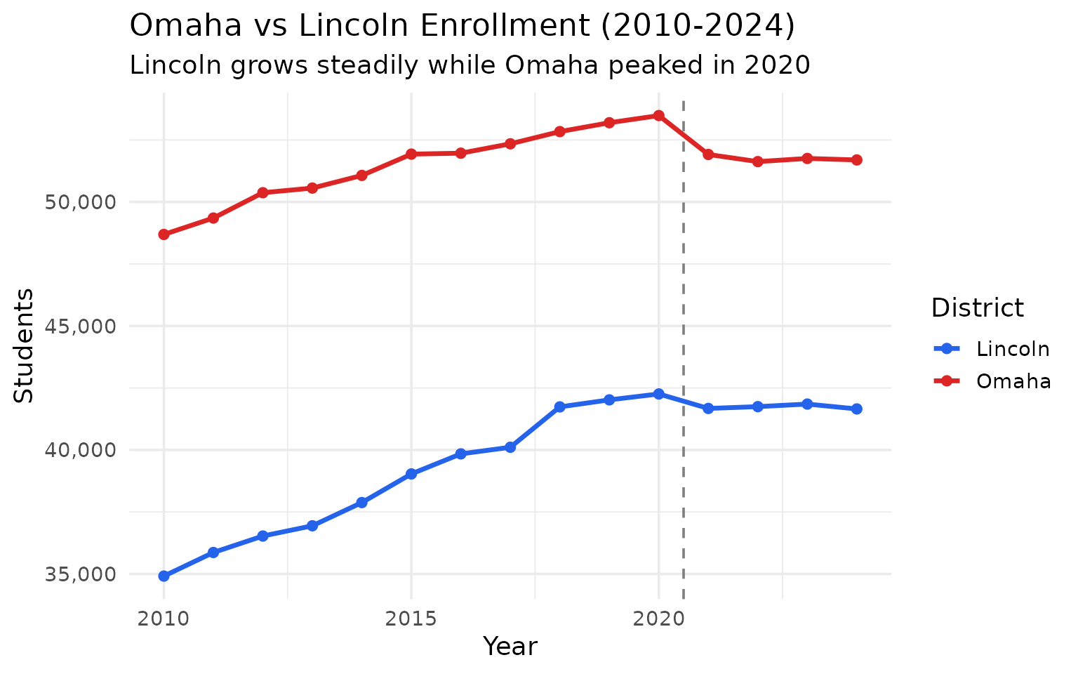
Lincoln is gaining on Omaha
Lincoln Public Schools added 6,740 students since 2010. The gap between the two districts narrowed from 13,775 to 10,039.
two_cities <- enr_multi %>%
  filter(is_district, subgroup == "total_enrollment", grade_level == "TOTAL",
         grepl("OMAHA PUBLIC|LINCOLN PUBLIC", district_name, ignore.case = TRUE)) %>%
  mutate(city = if_else(grepl("OMAHA", district_name, ignore.case = TRUE), "Omaha", "Lincoln")) %>%
  select(end_year, city, n_students)

stopifnot(nrow(two_cities) > 0)
two_cities %>%
  pivot_wider(names_from = city, values_from = n_students) %>%
  filter(end_year %in% c(2010, 2015, 2020, 2024)) %>%
  mutate(gap = Omaha - Lincoln)
#> # A tibble: 4 × 4
#>   end_year Omaha Lincoln   gap
#>      <dbl> <dbl>   <dbl> <dbl>
#> 1     2010 48689   34914 13775
#> 2     2015 51928   39034 12894
#> 3     2020 53483   42258 11225
#> 4     2024 51693   41654 10039
ggplot(two_cities, aes(x = end_year, y = n_students, color = city)) +
  geom_line(linewidth = 1.2) +
  geom_point(size = 2) +
  geom_vline(xintercept = 2020.5, linetype = "dashed", color = "gray50") +
  scale_y_continuous(labels = scales::comma) +
  scale_color_manual(values = c("Omaha" = "#dc2626", "Lincoln" = "#2563eb")) +
  labs(
    title = "Omaha vs Lincoln Enrollment (2010-2024)",
    subtitle = "Lincoln grows steadily while Omaha peaked in 2020",
    x = "Year",
    y = "Students",
    color = "District"
  )
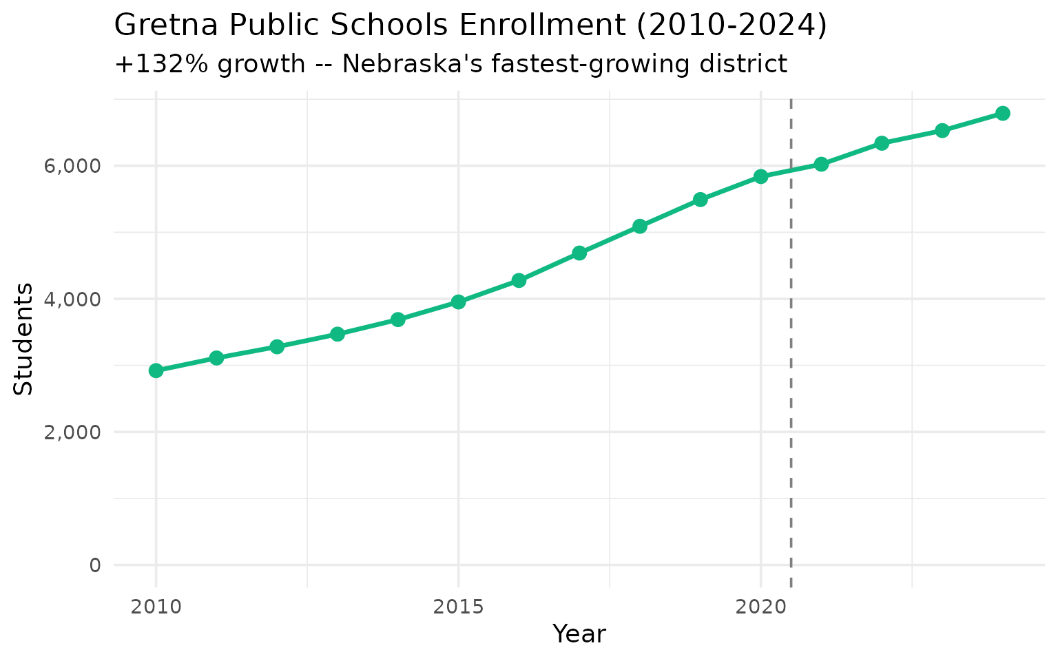
Gretna grew 132% since 2010 – Nebraska’s fastest-growing district
From 2,921 to 6,788 students, this Omaha-area suburb has more than doubled enrollment.
gretna <- enr_multi %>%
  filter(is_district, subgroup == "total_enrollment", grade_level == "TOTAL",
         district_name == "GRETNA PUBLIC SCHOOLS") %>%
  select(end_year, district_name, n_students)

stopifnot(nrow(gretna) > 0)
gretna %>%
  filter(end_year %in% c(2010, 2014, 2018, 2022, 2024))
#>   end_year         district_name n_students
#> 1     2010 GRETNA PUBLIC SCHOOLS       2921
#> 2     2014 GRETNA PUBLIC SCHOOLS       3688
#> 3     2018 GRETNA PUBLIC SCHOOLS       5090
#> 4     2022 GRETNA PUBLIC SCHOOLS       6339
#> 5     2024 GRETNA PUBLIC SCHOOLS       6788
ggplot(gretna, aes(x = end_year, y = n_students)) +
  geom_line(color = "#10b981", linewidth = 1.2) +
  geom_point(color = "#10b981", size = 3) +
  geom_vline(xintercept = 2020.5, linetype = "dashed", color = "gray50") +
  scale_y_continuous(labels = scales::comma, limits = c(0, NA)) +
  labs(
    title = "Gretna Public Schools Enrollment (2010-2024)",
    subtitle = "+132% growth -- Nebraska's fastest-growing district",
    x = "Year",
    y = "Students"
  )
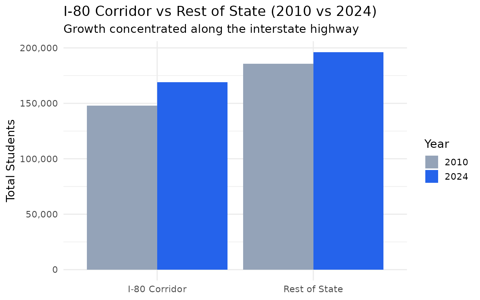
The I-80 corridor gained 21,000 students while the rest of the state grew too
Districts along Interstate 80 from Omaha to Kearney hold 46% of all students but captured most of the growth.
# Major I-80 districts: Omaha metro, Lincoln, Grand Island, Kearney
i80_patterns <- c("OMAHA", "LINCOLN", "MILLARD", "PAPILLION", "BELLEVUE",
                  "ELKHORN", "GRAND ISLAND", "KEARNEY")

i80_growth <- enr_multi %>%
  filter(is_district, subgroup == "total_enrollment", grade_level == "TOTAL",
         end_year %in% c(2010, 2024)) %>%
  rowwise() %>%
  mutate(is_i80 = any(sapply(i80_patterns, function(x) grepl(x, district_name, ignore.case = TRUE)))) %>%
  ungroup() %>%
  group_by(end_year, is_i80) %>%
  summarize(total = sum(n_students), n_districts = n(), .groups = "drop") %>%
  mutate(region = if_else(is_i80, "I-80 Corridor", "Rest of State"))

stopifnot(nrow(i80_growth) > 0)
i80_growth %>%
  select(end_year, region, total, n_districts) %>%
  pivot_wider(names_from = end_year, values_from = c(total, n_districts))
#> # A tibble: 2 × 5
#>   region        total_2010 total_2024 n_districts_2010 n_districts_2024
#>   <chr>              <dbl>      <dbl>            <int>            <int>
#> 1 Rest of State     185827     196252              439              402
#> 2 I-80 Corridor     148008     169215               24               21
i80_growth %>%
  ggplot(aes(x = region, y = total, fill = factor(end_year))) +
  geom_col(position = "dodge") +
  scale_y_continuous(labels = scales::comma) +
  scale_fill_manual(values = c("2010" = "#94a3b8", "2024" = "#2563eb")) +
  labs(
    title = "I-80 Corridor vs Rest of State (2010 vs 2024)",
    subtitle = "Growth concentrated along the interstate highway",
    x = NULL,
    y = "Total Students",
    fill = "Year"
  )
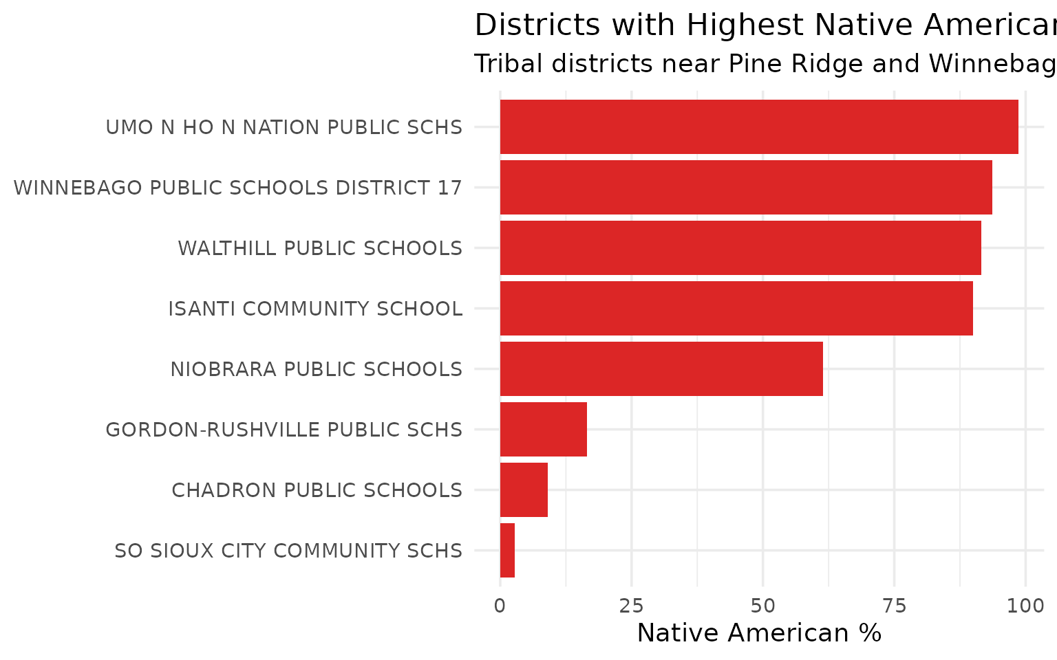
Tribal districts are 90-99% Native American
UMO N HO N NATION, WINNEBAGO, and WALTHILL serve predominantly Native American populations near Nebraska’s reservations.
# Look at districts with notable Native American populations
native_districts <- enr_2024 %>%
  filter(is_district, grade_level == "TOTAL",
         subgroup == "native_american") %>%
  arrange(desc(n_students)) %>%
  head(10) %>%
  select(district_name, n_students)

# Get total enrollment for these districts to calculate percentages
native_pct <- enr_2024 %>%
  filter(is_district, grade_level == "TOTAL",
         subgroup %in% c("total_enrollment", "native_american"),
         district_name %in% native_districts$district_name) %>%
  select(district_name, subgroup, n_students) %>%
  pivot_wider(names_from = subgroup, values_from = n_students) %>%
  mutate(pct = round(native_american / total_enrollment * 100, 1)) %>%
  arrange(desc(pct)) %>%
  head(8)

stopifnot(nrow(native_pct) > 0)
native_pct
#> # A tibble: 8 × 4
#>   district_name                        total_enrollment native_american   pct
#>   <chr>                                           <dbl>           <dbl> <dbl>
#> 1 UMO N HO N NATION PUBLIC SCHS                     664             655  98.6
#> 2 WINNEBAGO PUBLIC SCHOOLS DISTRICT 17              638             598  93.7
#> 3 WALTHILL PUBLIC SCHOOLS                           321             294  91.6
#> 4 ISANTI COMMUNITY SCHOOL                           229             206  90
#> 5 NIOBRARA PUBLIC SCHOOLS                           220             135  61.4
#> 6 GORDON-RUSHVILLE PUBLIC SCHS                      534              88  16.5
#> 7 CHADRON PUBLIC SCHOOLS                            971              87   9
#> 8 SO SIOUX CITY COMMUNITY SCHS                     3801             107   2.8
native_pct %>%
  mutate(district_name = reorder(district_name, pct)) %>%
  ggplot(aes(x = pct, y = district_name)) +
  geom_col(fill = "#dc2626") +
  labs(
    title = "Districts with Highest Native American Enrollment (2024)",
    subtitle = "Tribal districts near Pine Ridge and Winnebago reservations",
    x = "Native American %",
    y = NULL
  )
Session Info
sessionInfo()
#> R version 4.5.2 (2025-10-31)
#> Platform: x86_64-pc-linux-gnu
#> Running under: Ubuntu 24.04.3 LTS
#>
#> Matrix products: default
#> BLAS:   /usr/lib/x86_64-linux-gnu/openblas-pthread/libblas.so.3
#> LAPACK: /usr/lib/x86_64-linux-gnu/openblas-pthread/libopenblasp-r0.3.26.so;  LAPACK version 3.12.0
#>
#> locale:
#>  [1] LC_CTYPE=C.UTF-8       LC_NUMERIC=C           LC_TIME=C.UTF-8
#>  [4] LC_COLLATE=C.UTF-8     LC_MONETARY=C.UTF-8    LC_MESSAGES=C.UTF-8
#>  [7] LC_PAPER=C.UTF-8       LC_NAME=C              LC_ADDRESS=C
#> [10] LC_TELEPHONE=C         LC_MEASUREMENT=C.UTF-8 LC_IDENTIFICATION=C
#>
#> time zone: UTC
#> tzcode source: system (glibc)
#>
#> attached base packages:
#> [1] stats     graphics  grDevices utils     datasets  methods   base
#>
#> other attached packages:
#> [1] ggplot2_4.0.2      tidyr_1.3.2        dplyr_1.2.0        neschooldata_0.1.0
#>
#> loaded via a namespace (and not attached):
#>  [1] utf8_1.2.6         rappdirs_0.3.4     sass_0.4.10        generics_0.1.4
#>  [5] hms_1.1.4          digest_0.6.39      magrittr_2.0.4     evaluate_1.0.5
#>  [9] grid_4.5.2         RColorBrewer_1.1-3 fastmap_1.2.0      jsonlite_2.0.0
#> [13] httr_1.4.8         purrr_1.2.1        scales_1.4.0       codetools_0.2-20
#> [17] textshaping_1.0.5  jquerylib_0.1.4    cli_3.6.5          rlang_1.1.7
#> [21] crayon_1.5.3       bit64_4.6.0-1      withr_3.0.2        cachem_1.1.0
#> [25] yaml_2.3.12        tools_4.5.2        parallel_4.5.2     tzdb_0.5.0
#> [29] curl_7.0.0         vctrs_0.7.1        R6_2.6.1           lifecycle_1.0.5
#> [33] fs_1.6.7           bit_4.6.0          vroom_1.7.0        ragg_1.5.1
#> [37] pkgconfig_2.0.3    desc_1.4.3         pkgdown_2.2.0      pillar_1.11.1
#> [41] bslib_0.10.0       gtable_0.3.6       glue_1.8.0         systemfonts_1.3.2
#> [45] xfun_0.56          tibble_3.3.1       tidyselect_1.2.1   knitr_1.51
#> [49] farver_2.1.2       htmltools_0.5.9    rmarkdown_2.30     labeling_0.4.3
#> [53] readr_2.2.0        compiler_4.5.2     S7_0.2.1