15 Insights from Oregon School Enrollment Data
Source:vignettes/enrollment_hooks.Rmd
enrollment_hooks.Rmd
library(orschooldata)
library(dplyr)
library(tidyr)
library(ggplot2)

theme_set(theme_minimal(base_size = 14))
This vignette explores Oregon’s public school enrollment data, surfacing key trends across 15 years of data (2010-2024).
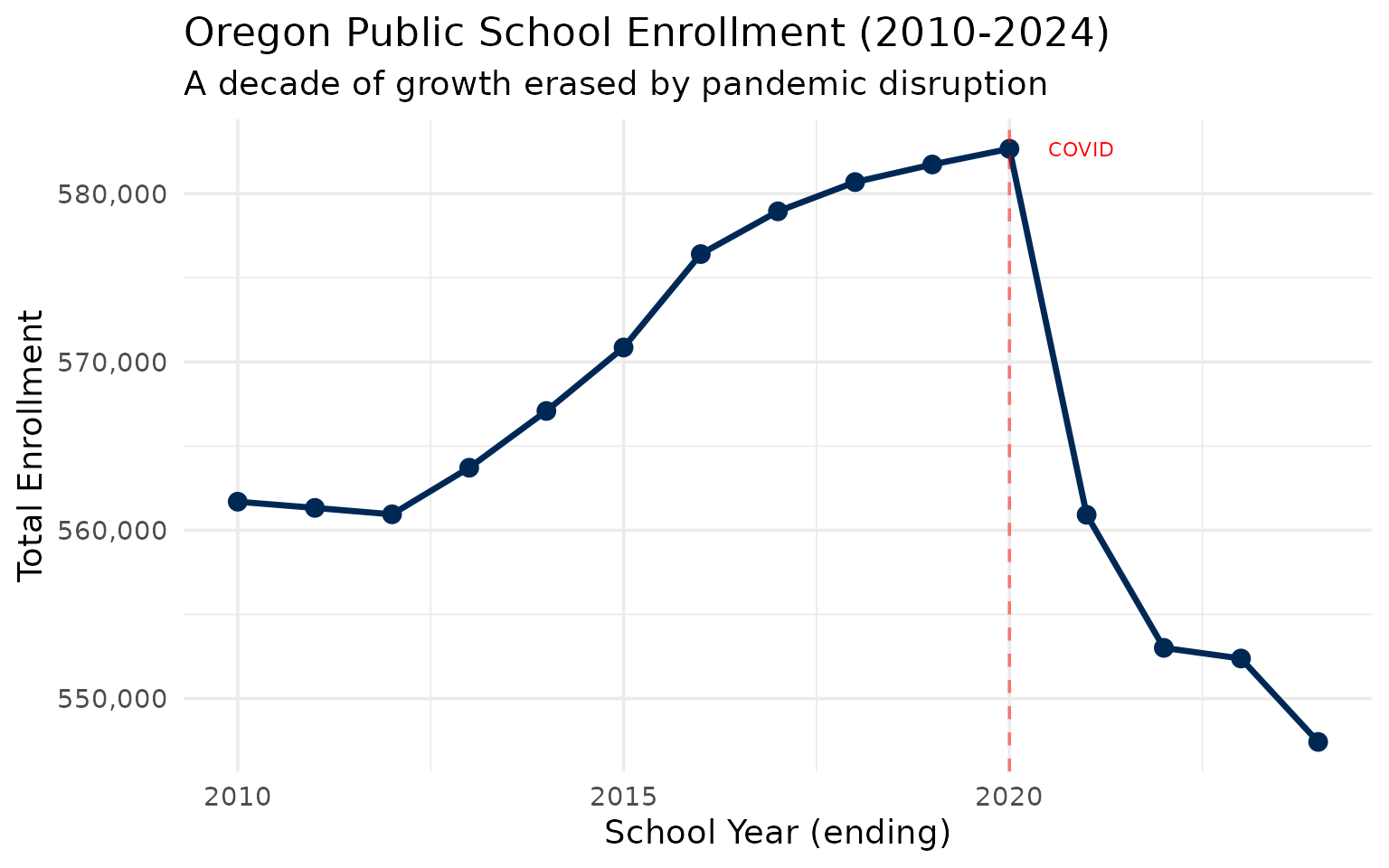
1. Oregon’s enrollment peaked in 2020, then COVID hit
The state added students for a decade, then lost nearly 22,000 in a single year during the pandemic.
enr <- fetch_enr_multi(2010:2024, use_cache = TRUE)

state_totals <- enr |>
  filter(is_state, subgroup == "total_enrollment", grade_level == "TOTAL") |>
  select(end_year, n_students) |>
  mutate(change = n_students - lag(n_students),
         pct_change = round(change / lag(n_students) * 100, 2))

stopifnot(nrow(state_totals) > 0)
state_totals
#>    end_year n_students change pct_change
#> 1      2010     561696     NA         NA
#> 2      2011     561328   -368      -0.07
#> 3      2012     560946   -382      -0.07
#> 4      2013     563714   2768       0.49
#> 5      2014     567086   3372       0.60
#> 6      2015     570857   3771       0.66
#> 7      2016     576407   5550       0.97
#> 8      2017     578947   2540       0.44
#> 9      2018     580684   1737       0.30
#> 10     2019     581730   1046       0.18
#> 11     2020     582661    931       0.16
#> 12     2021     560917 -21744      -3.73
#> 13     2022     553012  -7905      -1.41
#> 14     2023     552380   -632      -0.11
#> 15     2024     547424  -4956      -0.90
ggplot(state_totals, aes(x = end_year, y = n_students)) +
  geom_line(linewidth = 1.2, color = "#002855") +
  geom_point(size = 3, color = "#002855") +
  geom_vline(xintercept = 2020, linetype = "dashed", color = "red", alpha = 0.5) +
  annotate("text", x = 2020.5, y = max(state_totals$n_students, na.rm = TRUE),
           label = "COVID", hjust = 0, color = "red", size = 3) +
  scale_y_continuous(labels = scales::comma) +
  labs(
    title = "Oregon Public School Enrollment (2010-2024)",
    subtitle = "A decade of growth erased by pandemic disruption",
    x = "School Year (ending)",
    y = "Total Enrollment"
  )
2. Portland Public Schools lost 4,700 students since 2019
Oregon’s largest district peaked at 48,677 students in 2019 and has declined every year since, dropping to 90% of its peak by 2024.
portland <- enr |>
  filter(is_district, subgroup == "total_enrollment", grade_level == "TOTAL",
         district_id == "2180") |>
  select(end_year, district_name, n_students) |>
  mutate(pct_of_peak = round(n_students / max(n_students) * 100, 1))

stopifnot(nrow(portland) > 0)
portland
#>    end_year  district_name n_students pct_of_peak
#> 1      2010 Portland SD 1J      45678        93.8
#> 2      2011 Portland SD 1J      45718        93.9
#> 3      2012 Portland SD 1J      46190        94.9
#> 4      2013 Portland SD 1J      46581        95.7
#> 5      2014 Portland SD 1J      47099        96.8
#> 6      2015 Portland SD 1J      47647        97.9
#> 7      2016 Portland SD 1J      48383        99.4
#> 8      2017 Portland SD 1J      48198        99.0
#> 9      2018 Portland SD 1J      48650        99.9
#> 10     2019 Portland SD 1J      48677       100.0
#> 11     2020 Portland SD 1J      48559        99.8
#> 12     2021 Portland SD 1J      46924        96.4
#> 13     2022 Portland SD 1J      45123        92.7
#> 14     2023 Portland SD 1J      44681        91.8
#> 15     2024 Portland SD 1J      43979        90.3
top_districts <- enr |>
  filter(is_district, subgroup == "total_enrollment", grade_level == "TOTAL",
         end_year == 2024) |>
  arrange(desc(n_students)) |>
  head(5) |>
  pull(district_id)

stopifnot(length(top_districts) > 0)

enr |>
  filter(is_district, subgroup == "total_enrollment", grade_level == "TOTAL",
         district_id %in% top_districts) |>
  ggplot(aes(x = end_year, y = n_students, color = district_name)) +
  geom_line(linewidth = 1.2) +
  geom_point(size = 2) +
  scale_y_continuous(labels = scales::comma) +
  labs(
    title = "Oregon's Top 5 Districts: Enrollment Trends",
    subtitle = "Portland leads but is shrinking fastest",
    x = "School Year",
    y = "Enrollment",
    color = "District"
  ) +
  theme(legend.position = "bottom") +
  guides(color = guide_legend(nrow = 2))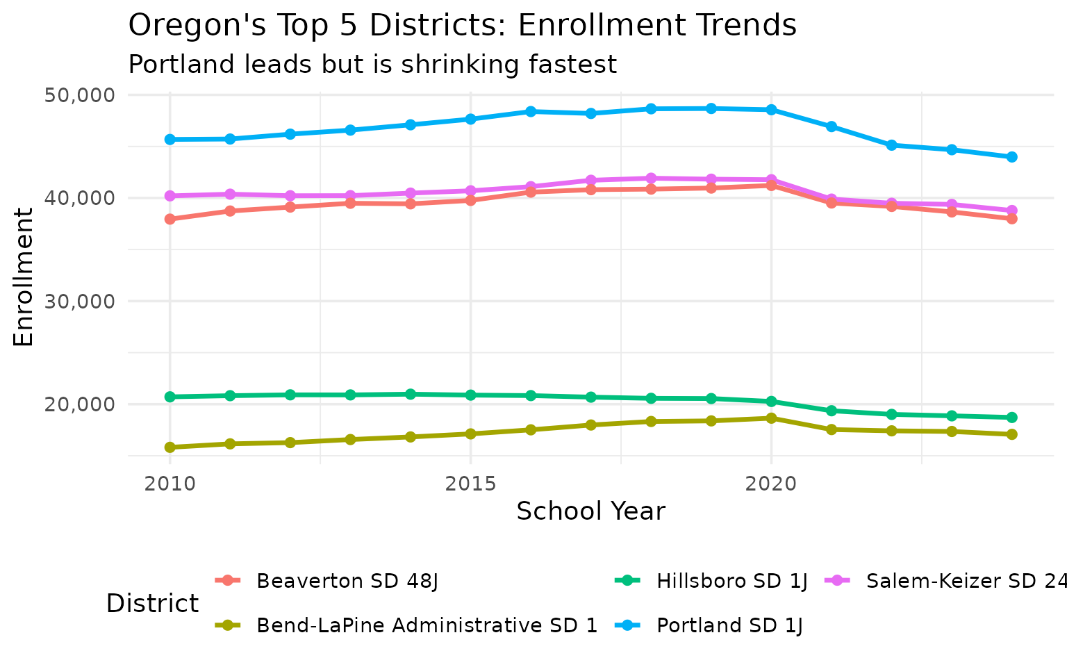
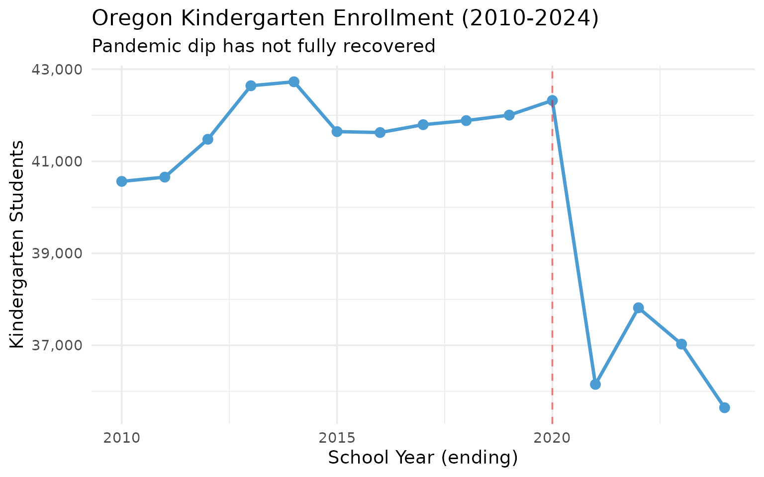
3. The COVID kindergarten collapse hasn’t recovered
Kindergarten enrollment dropped 14.6% from 2020 to 2021 and remains below pre-COVID levels, signaling smaller cohorts for years to come.
covid_grades <- enr |>
  filter(is_state, subgroup == "total_enrollment",
         grade_level %in% c("K", "01", "06", "09"),
         end_year %in% 2019:2024) |>
  select(end_year, grade_level, n_students) |>
  tidyr::pivot_wider(names_from = grade_level, values_from = n_students)

stopifnot(nrow(covid_grades) > 0)
covid_grades
#> # A tibble: 6 × 5
#>   end_year     K  `01`  `06`  `09`
#>      <int> <dbl> <dbl> <dbl> <dbl>
#> 1     2019 42004 42941 46655 45383
#> 2     2020 42322 42987 47024 45430
#> 3     2021 36151 40342 44012 46115
#> 4     2022 37816 38583 42274 46429
#> 5     2023 37026 40181 41907 46727
#> 6     2024 35644 38406 41670 44871
k_trend <- enr |>
  filter(is_state, subgroup == "total_enrollment", grade_level == "K")

stopifnot(nrow(k_trend) > 0)

k_trend |>
  ggplot(aes(x = end_year, y = n_students)) +
  geom_line(linewidth = 1.2, color = "#4B9CD3") +
  geom_point(size = 3, color = "#4B9CD3") +
  geom_vline(xintercept = 2020, linetype = "dashed", color = "red", alpha = 0.5) +
  scale_y_continuous(labels = scales::comma) +
  labs(
    title = "Oregon Kindergarten Enrollment (2010-2024)",
    subtitle = "Pandemic dip has not fully recovered",
    x = "School Year (ending)",
    y = "Kindergarten Students"
  )
4. High school grades are larger than elementary
Grade 9 enrollment exceeds kindergarten by several thousand students, reflecting the pandemic’s lasting impact on younger cohorts.
enr_2024 <- fetch_enr(2024, use_cache = TRUE)
grade_comparison <- enr_2024 |>
filter(is_state, subgroup == "total_enrollment",
grade_level %in% c("K", "01", "02", "03", "09", "10", "11", "12")) |>
select(grade_level, n_students) |>
arrange(grade_level)
stopifnot(nrow(grade_comparison) > 0)
grade_comparison
#> grade_level n_students
#> 1 01 38406
#> 2 02 40577
#> 3 03 40026
#> 4 09 44871
#> 5 10 46733
#> 6 11 45424
#> 7 12 46162
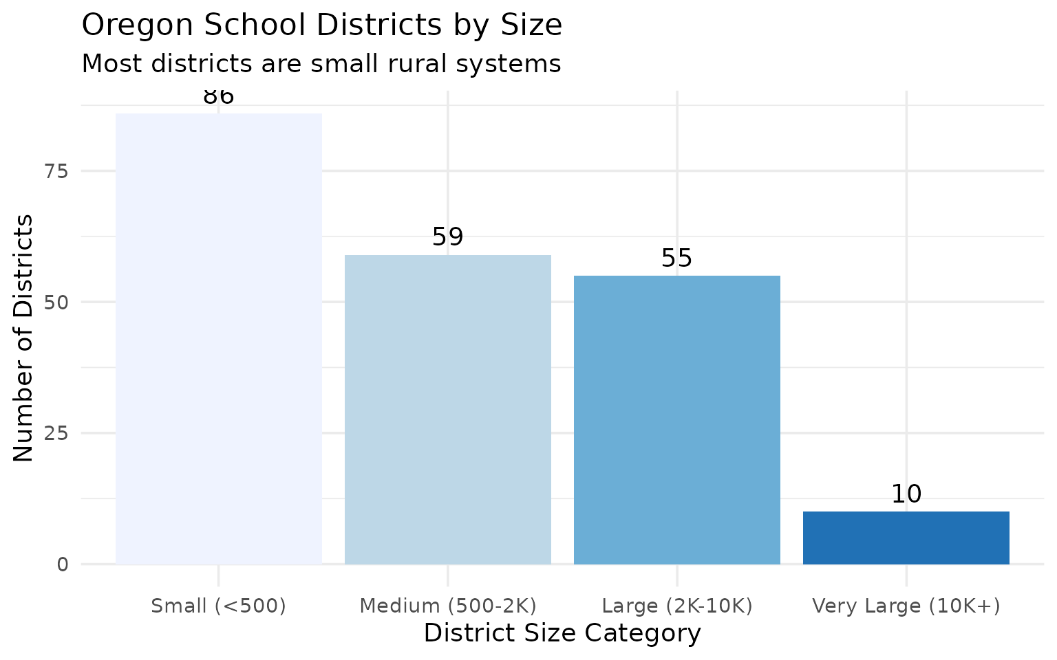
#> 8 K 356445. 86 districts have fewer than 500 students
Rural Oregon is vast, and many small districts serve tiny populations spread across large geographic areas.
district_sizes <- enr_2024 |>
  filter(is_district, subgroup == "total_enrollment", grade_level == "TOTAL") |>
  mutate(size_bucket = case_when(
    n_students < 500 ~ "Small (<500)",
    n_students < 2000 ~ "Medium (500-2K)",
    n_students < 10000 ~ "Large (2K-10K)",
    TRUE ~ "Very Large (10K+)"
  )) |>
  count(size_bucket)

stopifnot(nrow(district_sizes) > 0)
district_sizes
#>         size_bucket  n
#> 1    Large (2K-10K) 55
#> 2   Medium (500-2K) 59
#> 3      Small (<500) 86
#> 4 Very Large (10K+) 10
district_sizes |>
  mutate(size_bucket = factor(size_bucket,
         levels = c("Small (<500)", "Medium (500-2K)", "Large (2K-10K)", "Very Large (10K+)"))) |>
  ggplot(aes(x = size_bucket, y = n, fill = size_bucket)) +
  geom_col(show.legend = FALSE) +
  geom_text(aes(label = n), vjust = -0.5) +
  scale_fill_brewer(palette = "Blues") +
  labs(
    title = "Oregon School Districts by Size",
    subtitle = "Most districts are small rural systems",
    x = "District Size Category",
    y = "Number of Districts"
  )
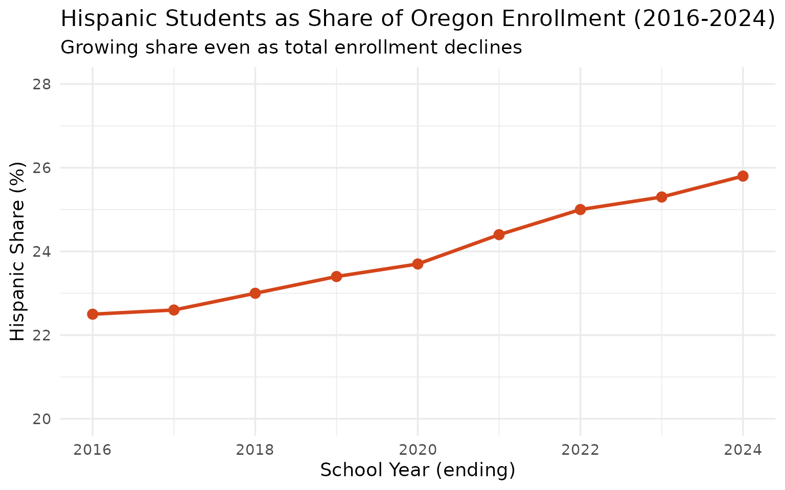
6. Oregon’s Hispanic student share rose from 22.5% to 25.8% in eight years
While total enrollment fell after 2020, Hispanic enrollment grew to 141,060 students—now more than one in four Oregon students.
hispanic_share <- enr |>
  filter(is_state, grade_level == "TOTAL",
         subgroup %in% c("total_enrollment", "hispanic")) |>
  select(end_year, subgroup, n_students) |>
  tidyr::pivot_wider(names_from = subgroup, values_from = n_students) |>
  filter(!is.na(hispanic)) |>
  mutate(hispanic_pct = round(hispanic / total_enrollment * 100, 1))

stopifnot(nrow(hispanic_share) > 0)
hispanic_share
#> # A tibble: 9 × 4
#>   end_year total_enrollment hispanic hispanic_pct
#>      <int>            <dbl>    <dbl>        <dbl>
#> 1     2016           576407   129410         22.5
#> 2     2017           578947   131089         22.6
#> 3     2018           580684   133822         23
#> 4     2019           581730   136186         23.4
#> 5     2020           582661   138273         23.7
#> 6     2021           560917   137101         24.4
#> 7     2022           553012   138112         25
#> 8     2023           552380   139928         25.3
#> 9     2024           547424   141060         25.8
ggplot(hispanic_share, aes(x = end_year, y = hispanic_pct)) +
  geom_line(linewidth = 1.2, color = "#D4451A") +
  geom_point(size = 3, color = "#D4451A") +
  scale_y_continuous(limits = c(20, 28)) +
  labs(
    title = "Hispanic Students as Share of Oregon Enrollment (2016-2024)",
    subtitle = "Growing share even as total enrollment declines",
    x = "School Year (ending)",
    y = "Hispanic Share (%)"
  )
7. Woodburn is 86% Hispanic—Oregon’s most concentrated district
Woodburn SD 103, south of Portland, has the highest Hispanic student share of any sizeable Oregon district at 86.1%.
hisp_districts <- enr_2024 |>
  filter(is_district, grade_level == "TOTAL",
         subgroup %in% c("total_enrollment", "hispanic")) |>
  select(district_name, subgroup, n_students) |>
  tidyr::pivot_wider(names_from = subgroup, values_from = n_students) |>
  mutate(hispanic_pct = round(hispanic / total_enrollment * 100, 1)) |>
  filter(total_enrollment >= 5000) |>
  arrange(desc(hispanic_pct))

stopifnot(nrow(hisp_districts) > 0)
hisp_districts
#> # A tibble: 27 × 4
#>    district_name          total_enrollment hispanic hispanic_pct
#>    <chr>                             <dbl>    <dbl>        <dbl>
#>  1 Woodburn SD 103                    5242     4514         86.1
#>  2 Hermiston SD 8                     5419     3256         60.1
#>  3 Forest Grove SD 15                 5809     3369         58
#>  4 Salem-Keizer SD 24J               38787    18050         46.5
#>  5 Reynolds SD 7                      9613     4229         44
#>  6 Hillsboro SD 1J                   18716     7725         41.3
#>  7 McMinnville SD 40                  6419     2436         37.9
#>  8 Gresham-Barlow SD 10J             11371     3768         33.1
#>  9 Centennial SD 28J                  5485     1755         32
#> 10 Tigard-Tualatin SD 23J            11620     3452         29.7
#> # ℹ 17 more rows
8. Portland SD 1J is Oregon’s largest district at 43,979 students
Portland leads Salem-Keizer by over 5,000 students, though both have declined since their pre-COVID peaks.
largest <- enr_2024 |>
  filter(is_district, subgroup == "total_enrollment", grade_level == "TOTAL") |>
  arrange(desc(n_students)) |>
  select(district_name, n_students) |>
  head(10)

stopifnot(nrow(largest) > 0)
largest
#>                      district_name n_students
#> 1                   Portland SD 1J      43979
#> 2              Salem-Keizer SD 24J      38787
#> 3                 Beaverton SD 48J      37988
#> 4                  Hillsboro SD 1J      18716
#> 5  Bend-LaPine Administrative SD 1      17075
#> 6            North Clackamas SD 12      16874
#> 7                     Eugene SD 4J      16318
#> 8                  Medford SD 549C      13750
#> 9           Tigard-Tualatin SD 23J      11620
#> 10           Gresham-Barlow SD 10J      11371
9. White students dropped from 63.4% to 58.4% of Oregon enrollment since 2016
Oregon is diversifying rapidly. White enrollment fell by 46,000 students while Hispanic and multiracial populations grew.
race_trend <- enr |>
  filter(is_state, grade_level == "TOTAL",
         subgroup %in% c("white", "hispanic", "multiracial", "asian", "black")) |>
  select(end_year, subgroup, n_students) |>
  filter(!is.na(n_students))

stopifnot(nrow(race_trend) > 0)

race_wide <- race_trend |>
  tidyr::pivot_wider(names_from = subgroup, values_from = n_students)

race_wide
#> # A tibble: 9 × 6
#>   end_year asian black hispanic  white multiracial
#>      <int> <dbl> <dbl>    <dbl>  <dbl>       <dbl>
#> 1     2016 22726 13744   129410 365593       32597
#> 2     2017 23067 13654   131089 364581       34200
#> 3     2018 23324 13509   133822 362396       35677
#> 4     2019 23267 13301   136186 360197       37136
#> 5     2020 23208 13176   138273 358257       38306
#> 6     2021 22733 13021   137101 338528       38629
#> 7     2022 22145 12731   138112 329994       39219
#> 8     2023 22181 12982   139928 326100       40024
#> 9     2024 22288 13114   141060 319798       40294
race_trend |>
  ggplot(aes(x = end_year, y = n_students, color = subgroup)) +
  geom_line(linewidth = 1.2) +
  geom_point(size = 2) +
  scale_y_continuous(labels = scales::comma) +
  scale_color_brewer(palette = "Set1") +
  labs(
    title = "Oregon Enrollment by Race/Ethnicity (2016-2024)",
    subtitle = "White enrollment declining, Hispanic and multiracial growing",
    x = "School Year (ending)",
    y = "Students",
    color = "Subgroup"
  ) +
  theme(legend.position = "bottom")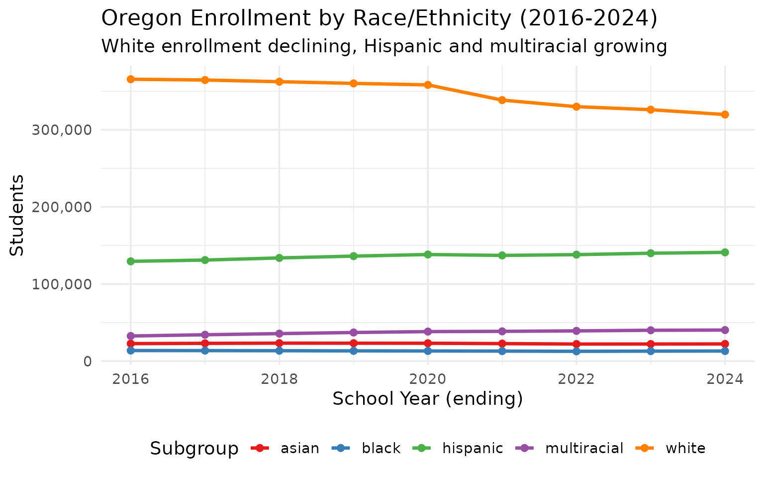
10. 15 years of data reveal long-term shifts
Oregon’s enrollment data spans from 2010 to 2024, capturing the Great Recession recovery, pre-pandemic growth, COVID disruption, and early recovery.
decade_summary <- enr |>
filter(is_state, subgroup == "total_enrollment", grade_level == "TOTAL",
end_year %in% c(2010, 2015, 2020, 2021, 2024)) |>
select(end_year, n_students) |>
mutate(label = case_when(
end_year == 2010 ~ "Post-recession",
end_year == 2015 ~ "Mid-decade",
end_year == 2020 ~ "Pre-COVID peak",
end_year == 2021 ~ "COVID low",
end_year == 2024 ~ "Current"
))
stopifnot(nrow(decade_summary) > 0)
decade_summary
#> end_year n_students label
#> 1 2010 561696 Post-recession
#> 2 2015 570857 Mid-decade
#> 3 2020 582661 Pre-COVID peak
#> 4 2021 560917 COVID low
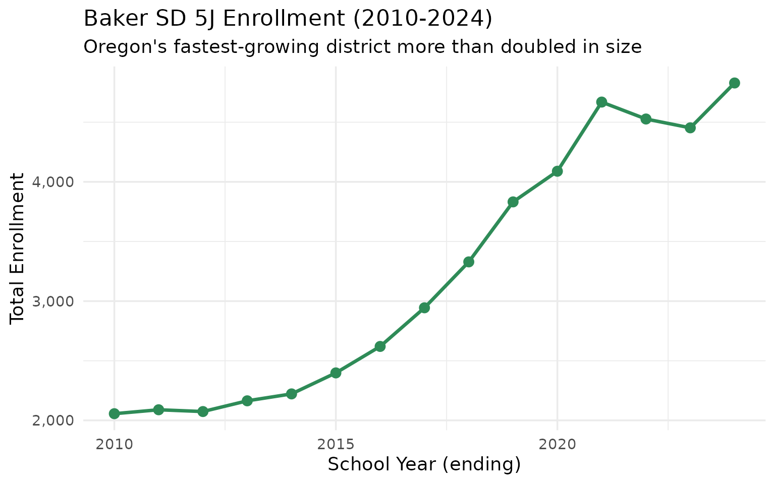
#> 5 2024 547424 Current11. Baker SD 5J more than doubled enrollment since 2010
Baker SD 5J grew from 2,056 to 4,829 students—a 135% increase—making it Oregon’s fastest-growing district by percentage.
baker <- enr |>
  filter(is_district, subgroup == "total_enrollment", grade_level == "TOTAL",
         district_id == "1894") |>
  select(end_year, district_name, n_students)

stopifnot(nrow(baker) > 0)
baker
#>    end_year district_name n_students
#> 1      2010   Baker SD 5J       2056
#> 2      2011   Baker SD 5J       2089
#> 3      2012   Baker SD 5J       2074
#> 4      2013   Baker SD 5J       2164
#> 5      2014   Baker SD 5J       2222
#> 6      2015   Baker SD 5J       2398
#> 7      2016   Baker SD 5J       2620
#> 8      2017   Baker SD 5J       2944
#> 9      2018   Baker SD 5J       3329
#> 10     2019   Baker SD 5J       3832
#> 11     2020   Baker SD 5J       4089
#> 12     2021   Baker SD 5J       4669
#> 13     2022   Baker SD 5J       4527
#> 14     2023   Baker SD 5J       4453
#> 15     2024   Baker SD 5J       4829
ggplot(baker, aes(x = end_year, y = n_students)) +
  geom_line(linewidth = 1.2, color = "#2E8B57") +
  geom_point(size = 3, color = "#2E8B57") +
  scale_y_continuous(labels = scales::comma) +
  labs(
    title = "Baker SD 5J Enrollment (2010-2024)",
    subtitle = "Oregon's fastest-growing district more than doubled in size",
    x = "School Year (ending)",
    y = "Total Enrollment"
  )
12. Beaverton vs Hillsboro: Suburban rivals
Washington County’s two largest districts show different trajectories over the past decade.
wash_county <- enr |>
  filter(is_district, subgroup == "total_enrollment", grade_level == "TOTAL",
         district_name %in% c("Beaverton SD 48J", "Hillsboro SD 1J")) |>
  select(end_year, district_name, n_students)

stopifnot(nrow(wash_county) > 0)

wash_county |>
  filter(end_year %in% c(2010, 2015, 2020, 2024))
#>   end_year    district_name n_students
#> 1     2010  Hillsboro SD 1J      20714
#> 2     2010 Beaverton SD 48J      37950
#> 3     2015  Hillsboro SD 1J      20884
#> 4     2015 Beaverton SD 48J      39763
#> 5     2020  Hillsboro SD 1J      20269
#> 6     2020 Beaverton SD 48J      41215
#> 7     2024  Hillsboro SD 1J      18716
#> 8     2024 Beaverton SD 48J      37988
wash_county |>
  ggplot(aes(x = end_year, y = n_students, color = district_name)) +
  geom_line(linewidth = 1.5) +
  geom_point(size = 3) +
  scale_y_continuous(labels = scales::comma) +
  scale_color_manual(values = c("Beaverton SD 48J" = "#1e3d59", "Hillsboro SD 1J" = "#ff6e40")) +
  labs(
    title = "Washington County's Suburban Giants",
    subtitle = "Beaverton and Hillsboro: two paths through growth and COVID",
    x = "School Year (ending)",
    y = "Total Enrollment",
    color = "District"
  ) +
  theme(legend.position = "bottom")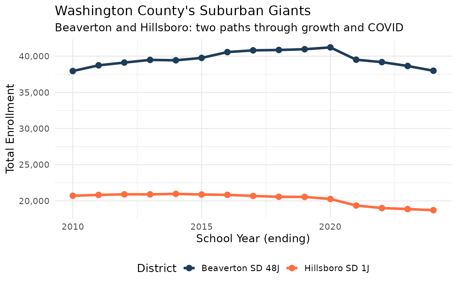
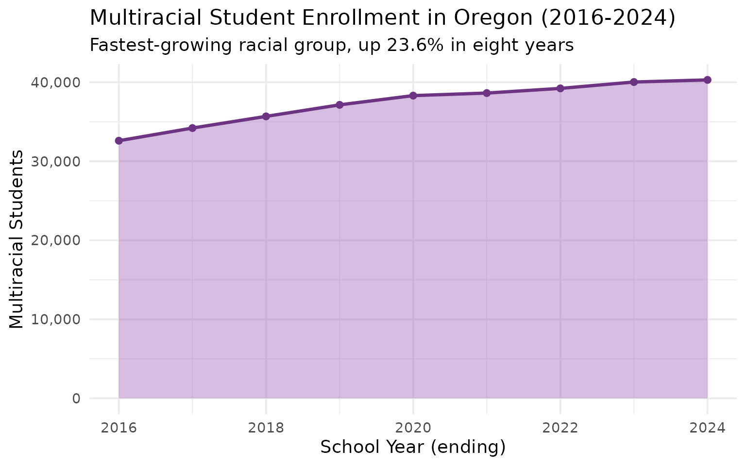
13. Multiracial is Oregon’s fastest-growing racial group
Multiracial students grew from 32,597 in 2016 to 40,294 in 2024—a 23.6% increase—even as total enrollment declined.
multi <- enr |>
  filter(is_state, grade_level == "TOTAL", subgroup == "multiracial") |>
  select(end_year, n_students) |>
  mutate(growth_from_2016 = round((n_students / first(n_students) - 1) * 100, 1))

stopifnot(nrow(multi) > 0)
multi
#>   end_year n_students growth_from_2016
#> 1     2016      32597              0.0
#> 2     2017      34200              4.9
#> 3     2018      35677              9.4
#> 4     2019      37136             13.9
#> 5     2020      38306             17.5
#> 6     2021      38629             18.5
#> 7     2022      39219             20.3
#> 8     2023      40024             22.8
#> 9     2024      40294             23.6
ggplot(multi, aes(x = end_year, y = n_students)) +
  geom_area(fill = "#9B59B6", alpha = 0.4) +
  geom_line(linewidth = 1.2, color = "#6C3483") +
  geom_point(size = 2, color = "#6C3483") +
  scale_y_continuous(labels = scales::comma) +
  labs(
    title = "Multiracial Student Enrollment in Oregon (2016-2024)",
    subtitle = "Fastest-growing racial group, up 23.6% in eight years",
    x = "School Year (ending)",
    y = "Multiracial Students"
  )
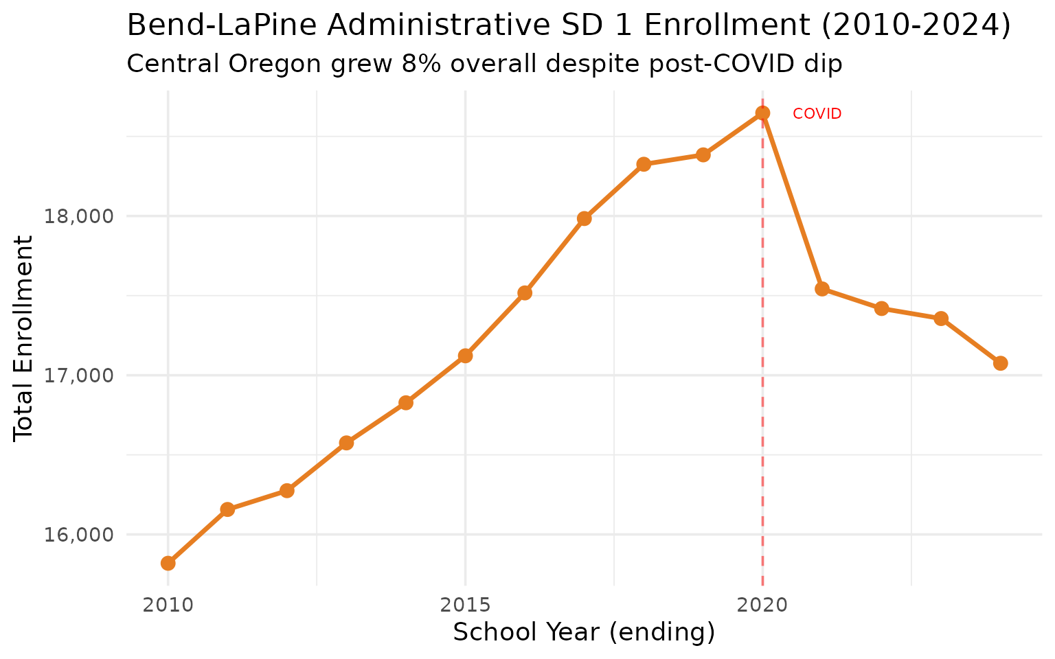
14. Bend-LaPine grew 8% while Portland shrank
Bend-LaPine Administrative SD 1 added over 1,200 students since 2010, bucking statewide post-COVID decline trends.
bend <- enr |>
  filter(is_district, subgroup == "total_enrollment", grade_level == "TOTAL",
         district_id == "1976") |>
  select(end_year, district_name, n_students)

stopifnot(nrow(bend) > 0)
bend
#>    end_year                   district_name n_students
#> 1      2010 Bend-LaPine Administrative SD 1      15819
#> 2      2011 Bend-LaPine Administrative SD 1      16157
#> 3      2012 Bend-LaPine Administrative SD 1      16275
#> 4      2013 Bend-LaPine Administrative SD 1      16575
#> 5      2014 Bend-LaPine Administrative SD 1      16827
#> 6      2015 Bend-LaPine Administrative SD 1      17122
#> 7      2016 Bend-LaPine Administrative SD 1      17517
#> 8      2017 Bend-LaPine Administrative SD 1      17984
#> 9      2018 Bend-LaPine Administrative SD 1      18325
#> 10     2019 Bend-LaPine Administrative SD 1      18384
#> 11     2020 Bend-LaPine Administrative SD 1      18647
#> 12     2021 Bend-LaPine Administrative SD 1      17542
#> 13     2022 Bend-LaPine Administrative SD 1      17419
#> 14     2023 Bend-LaPine Administrative SD 1      17356
#> 15     2024 Bend-LaPine Administrative SD 1      17075
ggplot(bend, aes(x = end_year, y = n_students)) +
  geom_line(linewidth = 1.2, color = "#E67E22") +
  geom_point(size = 3, color = "#E67E22") +
  geom_vline(xintercept = 2020, linetype = "dashed", color = "red", alpha = 0.5) +
  annotate("text", x = 2020.5, y = max(bend$n_students, na.rm = TRUE),
           label = "COVID", hjust = 0, color = "red", size = 3) +
  scale_y_continuous(labels = scales::comma) +
  labs(
    title = "Bend-LaPine Administrative SD 1 Enrollment (2010-2024)",
    subtitle = "Central Oregon grew 8% overall despite post-COVID dip",
    x = "School Year (ending)",
    y = "Total Enrollment"
  )
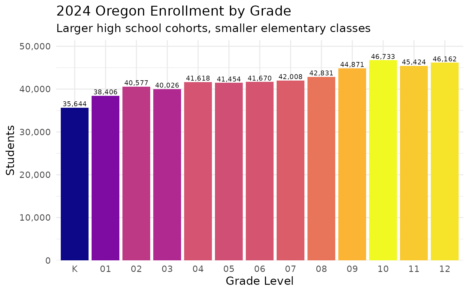
15. Grade-by-grade snapshot reveals demographic wave
Each grade level tells a story: today’s kindergartners are tomorrow’s high schoolers.
grade_snapshot <- enr |>
  filter(is_state, subgroup == "total_enrollment",
         grade_level %in% c("K", "01", "02", "03", "04", "05", "06", "07", "08", "09", "10", "11", "12"),
         end_year == 2024) |>
  select(grade_level, n_students) |>
  arrange(grade_level)

stopifnot(nrow(grade_snapshot) > 0)
grade_snapshot
#>    grade_level n_students
#> 1           01      38406
#> 2           02      40577
#> 3           03      40026
#> 4           04      41618
#> 5           05      41454
#> 6           06      41670
#> 7           07      42008
#> 8           08      42831
#> 9           09      44871
#> 10          10      46733
#> 11          11      45424
#> 12          12      46162
#> 13           K      35644
grade_snapshot |>
  mutate(grade_level = factor(grade_level, levels = c("K", sprintf("%02d", 1:12)))) |>
  ggplot(aes(x = grade_level, y = n_students, fill = n_students)) +
  geom_col() +
  geom_text(aes(label = scales::comma(n_students)), vjust = -0.3, size = 3) +
  scale_y_continuous(labels = scales::comma, expand = expansion(mult = c(0, 0.1))) +
  scale_fill_viridis_c(option = "plasma", guide = "none") +
  labs(
    title = "2024 Oregon Enrollment by Grade",
    subtitle = "Larger high school cohorts, smaller elementary classes",
    x = "Grade Level",
    y = "Students"
  )
Summary
Oregon’s school enrollment data reveals: - Pandemic disruption: Enrollment peaked in 2020 and is still declining - Urban decline: Portland Public Schools lost nearly 5,000 students since 2019 - Rural challenges: 86 districts have fewer than 500 students - Demographic shift: Hispanic students now 25.8% of enrollment, up from 22.5% in 2016 - Kindergarten gap: COVID’s impact on youngest cohorts persists - Diversifying state: White enrollment dropped 5 percentage points since 2016 - Suburban divergence: Beaverton and Hillsboro on different growth paths - Multiracial growth: Fastest-growing racial group, up 23.6% since 2016 - Central Oregon boom: Bend-LaPine grew 8% while the state shrank - Grade-level dynamics: High school cohorts larger than elementary
These patterns shape school funding, facility planning, and staffing decisions across the Beaver State.
Data sourced from the Oregon Department of Education Fall Membership Reports.
Session Info
sessionInfo()
#> R version 4.5.2 (2025-10-31)
#> Platform: x86_64-pc-linux-gnu
#> Running under: Ubuntu 24.04.3 LTS
#>
#> Matrix products: default
#> BLAS:   /usr/lib/x86_64-linux-gnu/openblas-pthread/libblas.so.3
#> LAPACK: /usr/lib/x86_64-linux-gnu/openblas-pthread/libopenblasp-r0.3.26.so;  LAPACK version 3.12.0
#>
#> locale:
#>  [1] LC_CTYPE=C.UTF-8       LC_NUMERIC=C           LC_TIME=C.UTF-8
#>  [4] LC_COLLATE=C.UTF-8     LC_MONETARY=C.UTF-8    LC_MESSAGES=C.UTF-8
#>  [7] LC_PAPER=C.UTF-8       LC_NAME=C              LC_ADDRESS=C
#> [10] LC_TELEPHONE=C         LC_MEASUREMENT=C.UTF-8 LC_IDENTIFICATION=C
#>
#> time zone: UTC
#> tzcode source: system (glibc)
#>
#> attached base packages:
#> [1] stats     graphics  grDevices utils     datasets  methods   base
#>
#> other attached packages:
#> [1] ggplot2_4.0.2      tidyr_1.3.2        dplyr_1.2.0        orschooldata_0.1.0
#>
#> loaded via a namespace (and not attached):
#>  [1] gtable_0.3.6       jsonlite_2.0.0     compiler_4.5.2     tidyselect_1.2.1
#>  [5] jquerylib_0.1.4    systemfonts_1.3.2  scales_1.4.0       textshaping_1.0.5
#>  [9] readxl_1.4.5       yaml_2.3.12        fastmap_1.2.0      R6_2.6.1
#> [13] labeling_0.4.3     generics_0.1.4     curl_7.0.0         knitr_1.51
#> [17] tibble_3.3.1       desc_1.4.3         bslib_0.10.0       pillar_1.11.1
#> [21] RColorBrewer_1.1-3 rlang_1.1.7        utf8_1.2.6         cachem_1.1.0
#> [25] xfun_0.56          fs_1.6.7           sass_0.4.10        S7_0.2.1
#> [29] viridisLite_0.4.3  cli_3.6.5          withr_3.0.2        pkgdown_2.2.0
#> [33] magrittr_2.0.4     digest_0.6.39      grid_4.5.2         rappdirs_0.3.4
#> [37] lifecycle_1.0.5    vctrs_0.7.1        evaluate_1.0.5     glue_1.8.0
#> [41] cellranger_1.1.0   farver_2.1.2       codetools_0.2-20   ragg_1.5.1
#> [45] httr_1.4.8         rmarkdown_2.30     purrr_1.2.1        tools_4.5.2
#> [49] pkgconfig_2.0.3    htmltools_0.5.9