scschooldata

Fetch and analyze South Carolina school enrollment data from the South Carolina Department of Education (SCDE) in R or Python. Over a decade of data (2013-2025) for every school, district, and the state – nearly 800,000 students across 80 districts.

Part of the state schooldata project, inspired by njschooldata – the original package that started this effort to make state education data accessible.

Full documentation – all 15 stories with interactive charts, getting-started guide, and complete function reference.

Highlights

library(scschooldata)
library(dplyr)
library(tidyr)
library(ggplot2)

theme_set(theme_minimal(base_size = 14))

1. Kindergarten has not recovered from COVID

Kindergarten enrollment dropped sharply during the pandemic and has not returned to pre-pandemic levels, declining each year since a partial rebound in 2022.

k_enr <- fetch_enr_multi(2019:2025, use_cache = TRUE)

k_trends <- k_enr |>
  filter(is_state, subgroup == "total_enrollment", grade_level == "K") |>
  select(end_year, n_students) |>
  mutate(
    change_from_2019 = n_students - first(n_students),
    pct_change = round(change_from_2019 / first(n_students) * 100, 1)
  )
stopifnot(nrow(k_trends) > 0)

k_trends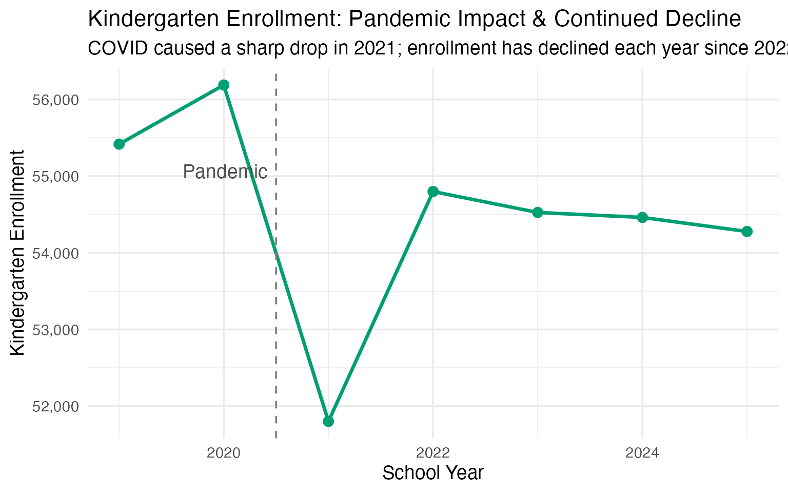

Kindergarten Enrollment: Pandemic Impact & Continued Decline

(source)

---

2. South Carolina’s racial composition is shifting fast

In just 8 years, the white share of enrollment has dropped from over 51% to under 48%, while Hispanic enrollment has surged from 9% to nearly 15%.

demo_enr <- fetch_enr_multi(c(2017, 2020, 2025), use_cache = TRUE)

demo_shift <- demo_enr |>
  filter(is_state, grade_level == "TOTAL",
         subgroup %in% c("white", "black", "hispanic", "multiracial")) |>
  select(end_year, subgroup, n_students) |>
  group_by(end_year) |>
  mutate(pct = round(n_students / sum(n_students, na.rm = TRUE) * 100, 1)) |>
  ungroup()
stopifnot(nrow(demo_shift) > 0)

demo_shift |>
  select(end_year, subgroup, n_students, pct) |>
  pivot_wider(names_from = end_year, values_from = c(n_students, pct))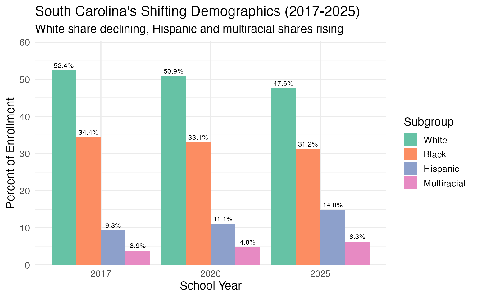

South Carolina’s Shifting Demographics (2017-2025)

(source)

---

3. State-authorized charters are growing fast

The SC Public Charter School District (code 900) serves state-authorized charter schools and has grown to over 21,000 students.

charter_enr <- fetch_enr_multi(c(2015, 2020, 2025), use_cache = TRUE)

charter_trends <- charter_enr |>
  filter(
    grepl("Charter School District", district_name),
    is_district,
    subgroup == "total_enrollment",
    grade_level == "TOTAL"
  ) |>
  select(end_year, n_students)
stopifnot(nrow(charter_trends) > 0)

charter_trends

enr_2025 <- fetch_enr(2025, use_cache = TRUE)

# Charter as percent of state
charter_pct <- enr_2025 |>
  filter(is_state | grepl("Charter School District", district_name),
         subgroup == "total_enrollment", grade_level == "TOTAL") |>
  select(district_name, n_students) |>
  mutate(type = ifelse(is.na(district_name), "State Total", "Charter")) |>
  select(type, n_students)

charter_pct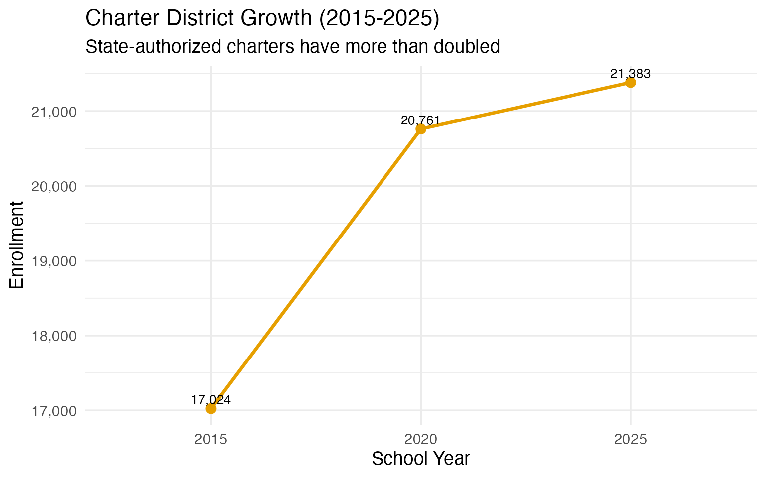

Charter District Growth (2015-2025)

(source)

---

Data Taxonomy

Category	Years	Function	Details
Enrollment	2013-2025	fetch_enr() / fetch_enr_multi()	State, district, school. Race, gender, econ disadv
Assessments	—	—	Not yet available
Graduation	—	—	Not yet available
Directory	2018-2025	fetch_directory()	School, district. Principal, superintendent, address, phone, website
Per-Pupil Spending	—	—	Not yet available
Accountability	—	—	Not yet available
Chronic Absence	—	—	Not yet available
EL Progress	—	—	Not yet available
Special Ed	—	—	Not yet available

See the full data category taxonomy

Quick Start

R

# install.packages("devtools")
devtools::install_github("almartin82/scschooldata")

library(scschooldata)
library(dplyr)

# Get 2025 enrollment data (2024-25 school year)
enr <- fetch_enr(2025, use_cache = TRUE)

# Statewide total
enr |>
  filter(is_state, subgroup == "total_enrollment", grade_level == "TOTAL") |>
  pull(n_students)

# Top 10 districts
enr |>
  filter(is_district, subgroup == "total_enrollment", grade_level == "TOTAL") |>
  arrange(desc(n_students)) |>
  select(district_name, n_students) |>
  head(10)

# Get multiple years
enr_multi <- fetch_enr_multi(2020:2025, use_cache = TRUE)

Python

import pyscschooldata as sc

# Get 2025 enrollment data (2024-25 school year)
df = sc.fetch_enr(2025)

# Statewide total
state_total = df[(df['is_state'] == True) &
                 (df['subgroup'] == 'total_enrollment') &
                 (df['grade_level'] == 'TOTAL')]['n_students'].values[0]
print(f"Total enrollment: {state_total:,}")

# Top 10 districts
districts = df[(df['is_district'] == True) &
               (df['subgroup'] == 'total_enrollment') &
               (df['grade_level'] == 'TOTAL')]
print(districts.nlargest(10, 'n_students')[['district_name', 'n_students']])

# Get multiple years
df_multi = sc.fetch_enr_multi([2020, 2021, 2022, 2023, 2024, 2025])

Explore More

Full analysis with 15 stories: - Enrollment trends – 15 stories - Function reference

Data Notes

Source

Data is sourced directly from the South Carolina Department of Education Active Student Headcounts.

Available Years

• 2013-2025 (13 years of data)
• Data reflects the 45-day count (early fall enrollment snapshot)

Suppression Rules

South Carolina does not suppress small cell counts in the Active Student Headcounts data. All counts are reported as-is from the state.

Data Quality Notes

• School and district names may vary slightly across years
• Some schools open/close between years
• Charter schools are identified by is_charter = TRUE
• State-authorized charters are grouped under District 900 (SC Public Charter School District)

Census Day

The 45-day count typically occurs in late October/early November, representing enrollment approximately 45 school days into the academic year.

---

Deeper Dive

4. South Carolina is growing

Unlike many states facing enrollment decline, South Carolina has added approximately 40,000 students since 2015. The Palmetto State’s population growth is reflected in its schools.

enr <- fetch_enr_multi(c(2015, 2017, 2019, 2021, 2023, 2025), use_cache = TRUE)

state_totals <- enr |>
  filter(is_state, subgroup == "total_enrollment", grade_level == "TOTAL") |>
  select(end_year, n_students) |>
  mutate(
    change = n_students - lag(n_students),
    pct_change = round(change / lag(n_students) * 100, 2)
  )
stopifnot(nrow(state_totals) > 0)

state_totals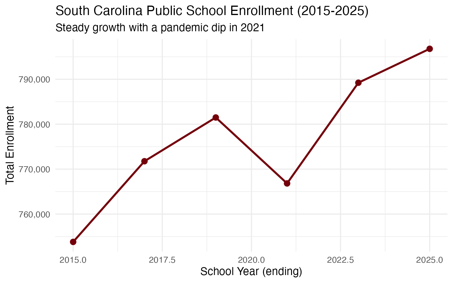

South Carolina Public School Enrollment (2015-2025)

(source)

---

5. Greenville County is the giant

Greenville County Schools enrolls nearly 77,000 students, making it the largest district in the state and one of the largest in the Southeast.

enr_2025 <- fetch_enr(2025, use_cache = TRUE)

top_districts <- enr_2025 |>
  filter(is_district, subgroup == "total_enrollment", grade_level == "TOTAL") |>
  arrange(desc(n_students)) |>
  head(10) |>
  select(district_name, n_students)
stopifnot(nrow(top_districts) > 0)

top_districts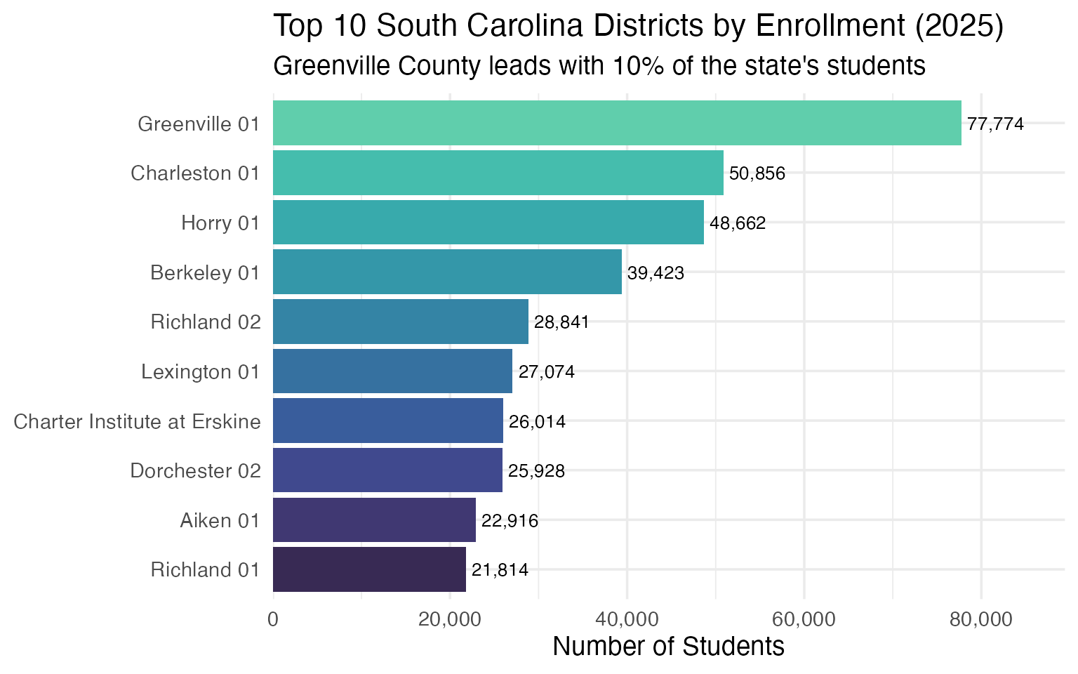

Top 10 South Carolina Districts by Enrollment (2025)

(source)

---

6. Hispanic enrollment is surging

Hispanic student enrollment has risen steadily, growing from about 10% in 2019 to over 14% of total enrollment in 2025.

demographics <- enr_2025 |>
  filter(is_state, grade_level == "TOTAL",
         subgroup %in% c("white", "black", "hispanic", "asian",
                         "native_american", "pacific_islander", "multiracial")) |>
  mutate(pct = round(n_students / sum(n_students, na.rm = TRUE) * 100, 1)) |>
  select(subgroup, n_students, pct) |>
  arrange(desc(n_students))
stopifnot(nrow(demographics) > 0)

demographics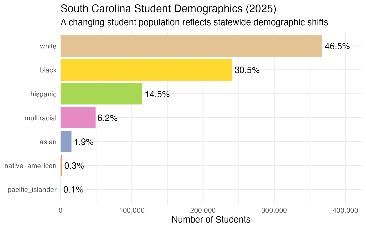

South Carolina Student Demographics (2025)

(source)

---

7. The I-85 Corridor is booming

Districts along the I-85 corridor from Greenville through Spartanburg are among the fastest-growing in the state, fueled by economic development and migration from other states.

i85_districts <- enr_2025 |>
  filter(
    grepl("Greenville|Spartanburg|Anderson", district_name),
    is_district,
    subgroup == "total_enrollment",
    grade_level == "TOTAL"
  ) |>
  arrange(desc(n_students)) |>
  select(district_name, n_students) |>
  head(8)
stopifnot(nrow(i85_districts) > 0)

i85_districts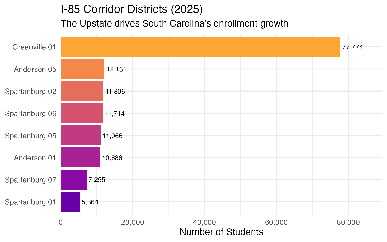

I-85 Corridor Districts (2025)

(source)

---

8. The Lowcountry is expanding

Charleston, Berkeley, and Dorchester counties form South Carolina’s tri-county Lowcountry region, and all three have seen substantial enrollment growth.

lowcountry_enr <- fetch_enr_multi(c(2015, 2020, 2025), use_cache = TRUE)

lowcountry <- lowcountry_enr |>
  filter(
    grepl("Charleston|Berkeley|Dorchester", district_name),
    is_district,
    subgroup == "total_enrollment",
    grade_level == "TOTAL"
  ) |>
  select(end_year, district_name, n_students) |>
  pivot_wider(names_from = end_year, values_from = n_students) |>
  mutate(
    growth = `2025` - `2015`,
    pct_growth = round(growth / `2015` * 100, 1)
  ) |>
  arrange(desc(growth))
stopifnot(nrow(lowcountry) > 0)

lowcountry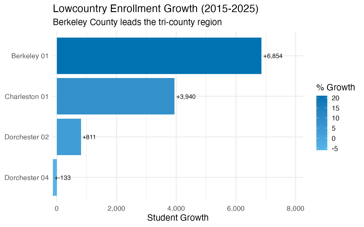

Lowcountry Enrollment Growth (2015-2025)

(source)

---

9. Rural Pee Dee districts are declining

While much of South Carolina grows, rural districts in the Pee Dee region face persistent enrollment decline.

pee_dee_enr <- fetch_enr_multi(c(2015, 2025), use_cache = TRUE)

pee_dee <- pee_dee_enr |>
  filter(
    grepl("Marion|Dillon|Marlboro|Florence", district_name),
    is_district,
    subgroup == "total_enrollment",
    grade_level == "TOTAL"
  ) |>
  select(end_year, district_name, n_students) |>
  pivot_wider(names_from = end_year, values_from = n_students) |>
  mutate(
    change = `2025` - `2015`,
    pct_change = round(change / `2015` * 100, 1)
  ) |>
  filter(!is.na(`2015`), !is.na(`2025`)) |>
  arrange(pct_change) |>
  head(8)
stopifnot(nrow(pee_dee) > 0)

pee_dee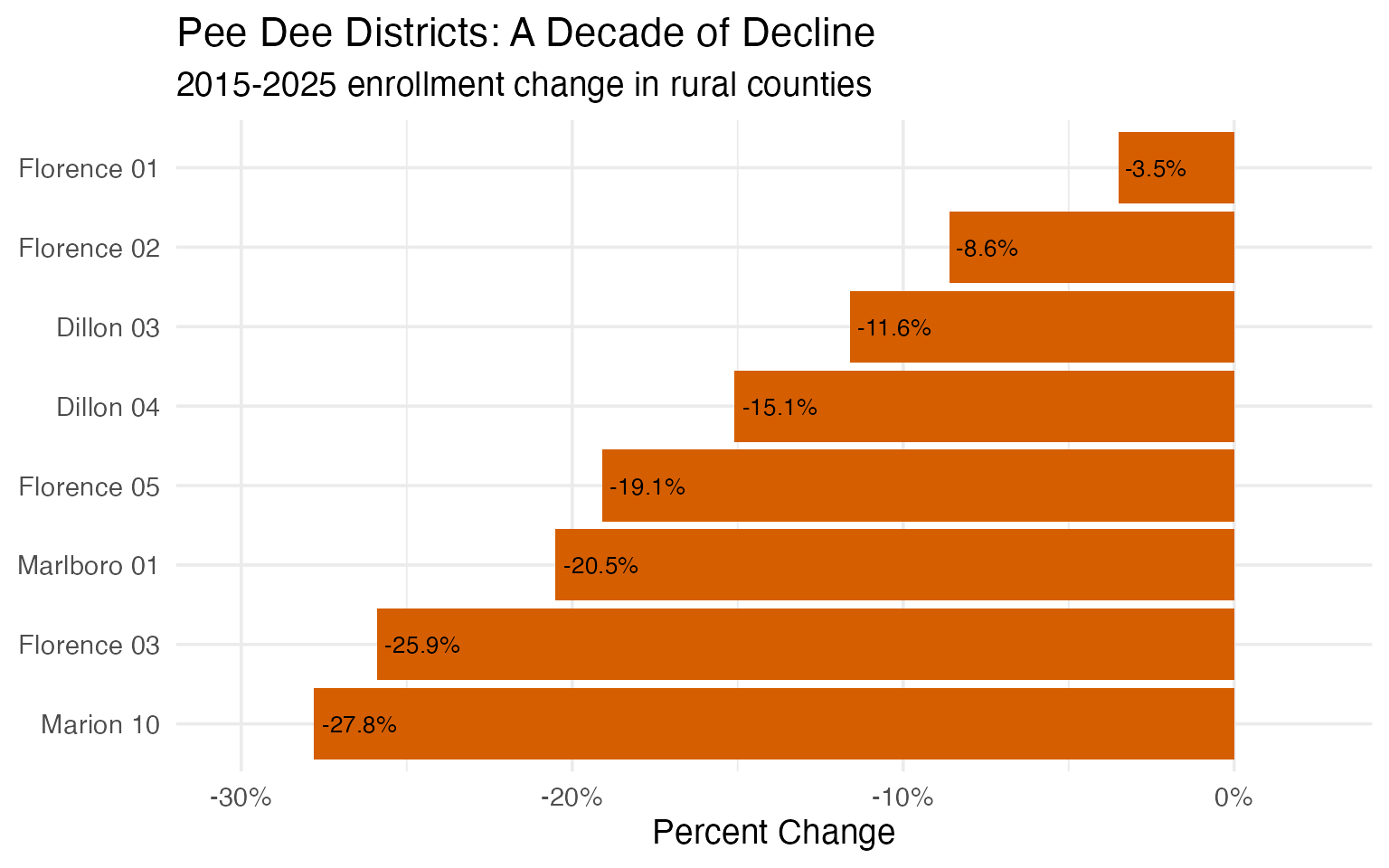

Pee Dee Districts: A Decade of Decline

(source)

---

10. District size varies dramatically

South Carolina’s 80 districts range from tiny rural systems to massive county-wide operations serving tens of thousands.

district_sizes <- enr_2025 |>
  filter(is_district, subgroup == "total_enrollment", grade_level == "TOTAL") |>
  mutate(size_bucket = case_when(
    n_students < 5000 ~ "Small (<5K)",
    n_students < 15000 ~ "Medium (5K-15K)",
    n_students < 30000 ~ "Large (15K-30K)",
    TRUE ~ "Very Large (30K+)"
  )) |>
  count(size_bucket) |>
  mutate(size_bucket = factor(size_bucket,
                              levels = c("Small (<5K)", "Medium (5K-15K)",
                                         "Large (15K-30K)", "Very Large (30K+)")))
stopifnot(nrow(district_sizes) > 0)

district_sizes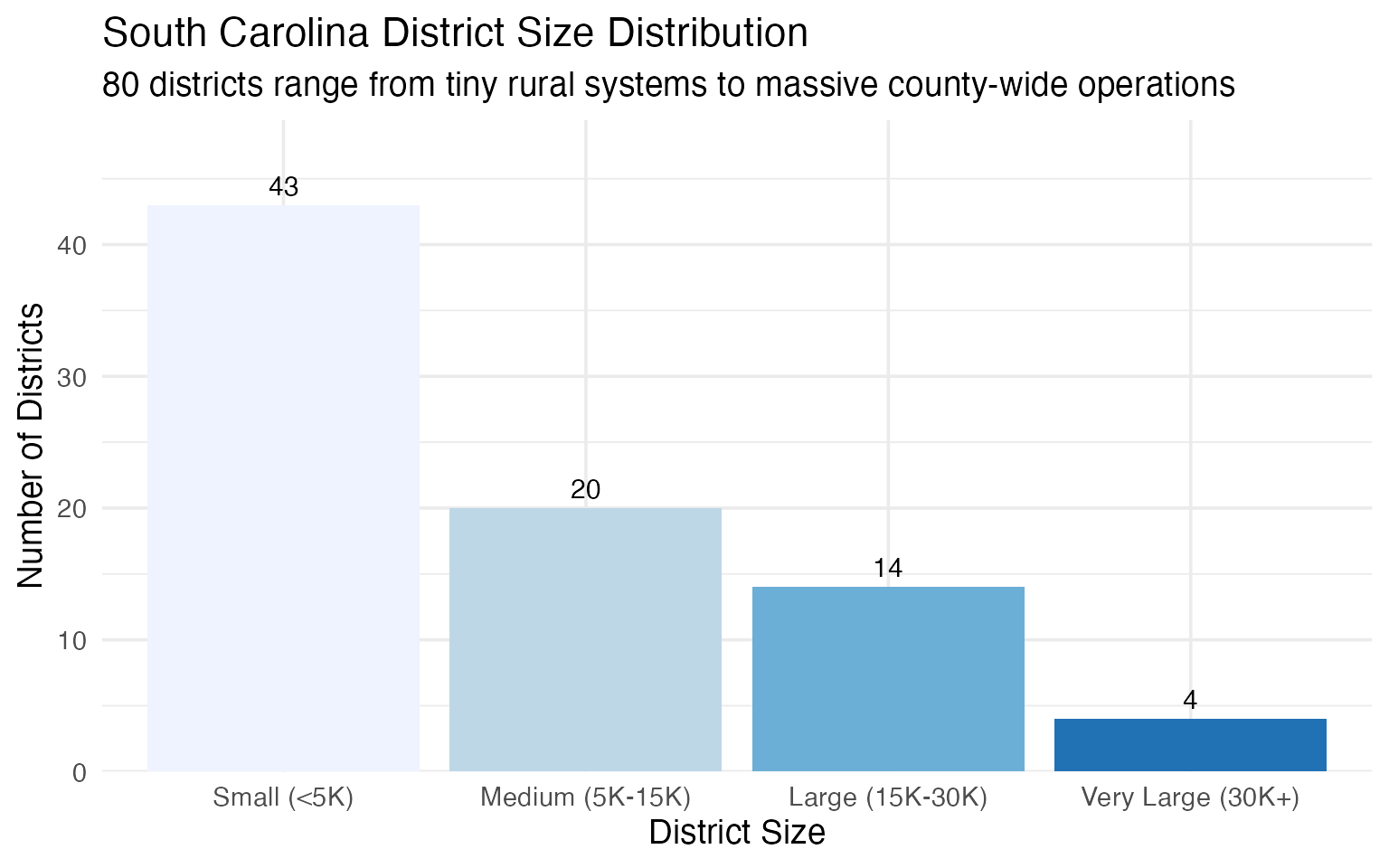

South Carolina District Size Distribution

(source)

---

11. Richland vs Lexington: Columbia’s Suburban Divide

The Columbia metro area is split between Richland and Lexington counties, with very different enrollment trajectories. Lexington County districts have grown substantially while Richland districts have been more stable.

columbia_enr <- fetch_enr_multi(c(2015, 2020, 2025), use_cache = TRUE)

columbia_districts <- columbia_enr |>
  filter(
    grepl("Richland|Lexington", district_name),
    is_district,
    subgroup == "total_enrollment",
    grade_level == "TOTAL"
  ) |>
  select(end_year, district_name, n_students) |>
  pivot_wider(names_from = end_year, values_from = n_students) |>
  mutate(
    growth = `2025` - `2015`,
    pct_growth = round(growth / `2015` * 100, 1),
    county = ifelse(grepl("Richland", district_name), "Richland", "Lexington")
  ) |>
  filter(!is.na(`2015`), !is.na(`2025`)) |>
  arrange(desc(growth))
stopifnot(nrow(columbia_districts) > 0)

columbia_districts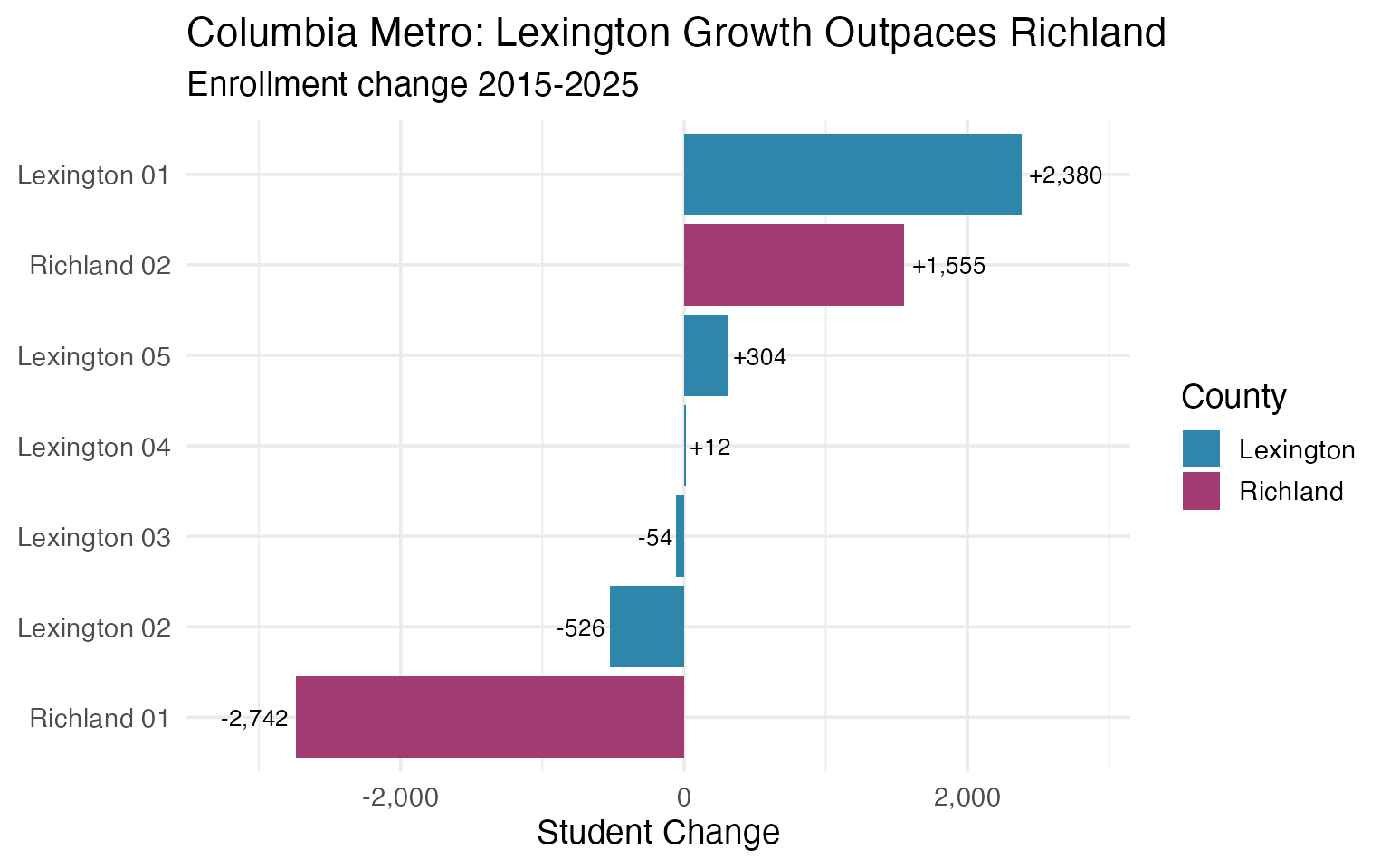

Columbia Metro: Lexington Growth Outpaces Richland

(source)

---

12. Boys slightly outnumber girls statewide

South Carolina enrolls slightly more male than female students overall, a pattern consistent across most large districts.

gender_data <- enr_2025 |>
  filter(
    is_district,
    subgroup %in% c("male", "female"),
    grade_level == "TOTAL"
  ) |>
  select(district_name, subgroup, n_students) |>
  pivot_wider(names_from = subgroup, values_from = n_students) |>
  filter(!is.na(male), !is.na(female)) |>
  mutate(
    total = male + female,
    pct_male = round(male / total * 100, 1)
  ) |>
  arrange(desc(total)) |>
  head(15)
stopifnot(nrow(gender_data) > 0)

gender_data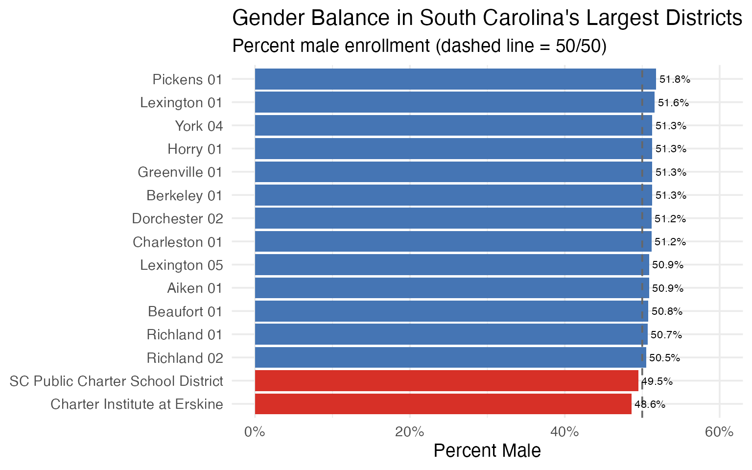

Gender Balance in South Carolina’s Largest Districts

(source)

---

13. High School Enrollment: The 9th Grade Bulge

High schools show a distinctive enrollment pattern: 9th grade is consistently the largest, with enrollment declining through 12th grade. This reflects retention, transfers, and dropouts.

hs_grades <- enr_2025 |>
  filter(
    is_state,
    subgroup == "total_enrollment",
    grade_level %in% c("09", "10", "11", "12")
  ) |>
  select(grade_level, n_students) |>
  mutate(
    grade_label = case_when(
      grade_level == "09" ~ "9th Grade",
      grade_level == "10" ~ "10th Grade",
      grade_level == "11" ~ "11th Grade",
      grade_level == "12" ~ "12th Grade"
    ),
    grade_label = factor(grade_label, levels = c("9th Grade", "10th Grade", "11th Grade", "12th Grade")),
    pct_of_9th = round(n_students / first(n_students) * 100, 1)
  )
stopifnot(nrow(hs_grades) > 0)

hs_grades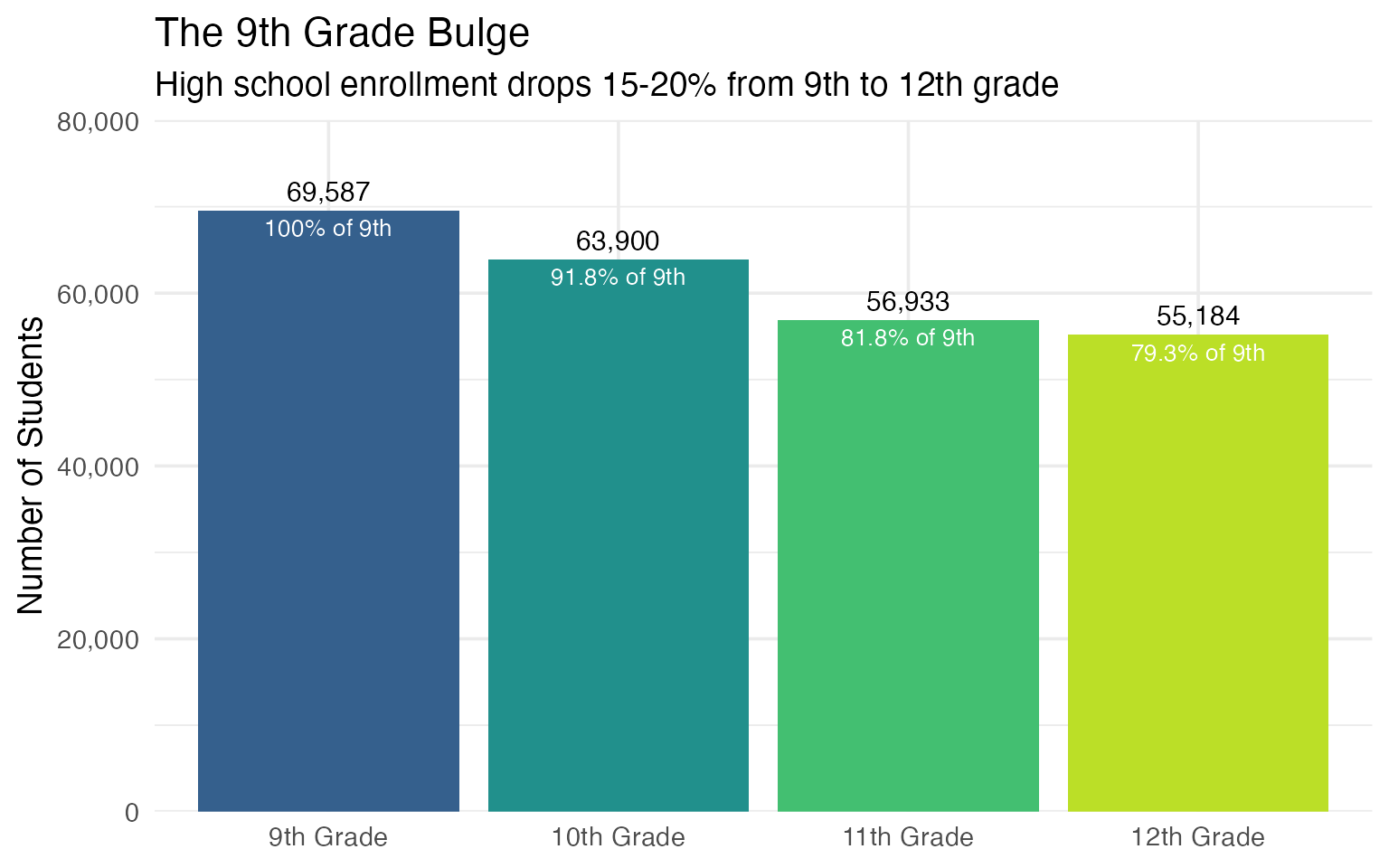

The 9th Grade Bulge

(source)

---

14. South Carolina’s Smallest Districts

Not all South Carolina districts are massive county systems. Several rural districts serve fewer than 2,000 students.

smallest <- enr_2025 |>
  filter(
    is_district,
    subgroup == "total_enrollment",
    grade_level == "TOTAL",
    !grepl("Charter", district_name)
  ) |>
  arrange(n_students) |>
  select(district_name, n_students) |>
  head(10)
stopifnot(nrow(smallest) > 0)

smallest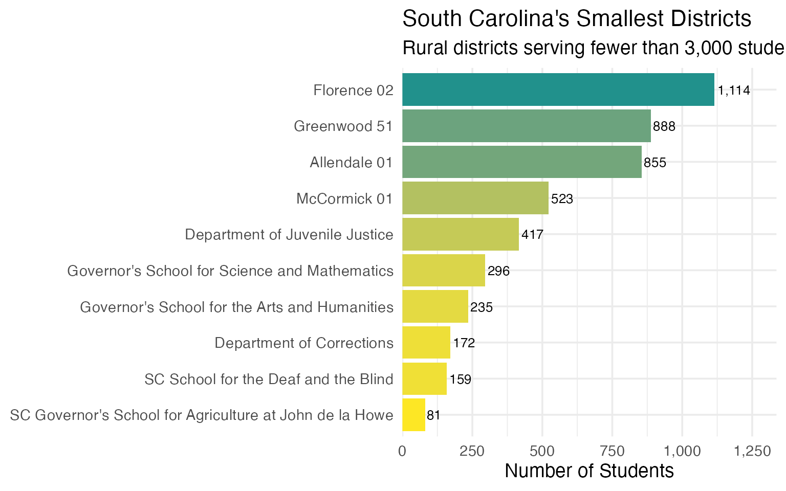

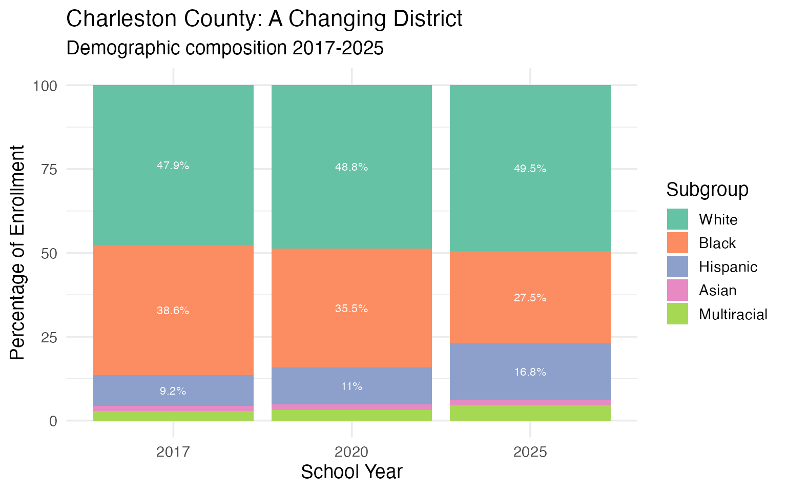
South Carolina’s Smallest Districts

(source)

---

15. Charleston’s Decade of Transformation

Charleston 01 (Charleston County) has undergone significant demographic change in recent years, reflecting the city’s rapid growth and gentrification.

charleston_demo <- fetch_enr_multi(c(2017, 2020, 2025), use_cache = TRUE)

charleston_demo_trends <- charleston_demo |>
  filter(
    grepl("Charleston", district_name),
    is_district,
    grade_level == "TOTAL",
    subgroup %in% c("white", "black", "hispanic", "asian", "multiracial")
  ) |>
  select(end_year, subgroup, n_students) |>
  group_by(end_year) |>
  mutate(pct = round(n_students / sum(n_students, na.rm = TRUE) * 100, 1)) |>
  ungroup()
stopifnot(nrow(charleston_demo_trends) > 0)

charleston_demo_trends |>
  pivot_wider(names_from = end_year, values_from = c(n_students, pct))

Charleston County: A Changing District

(source)