15 Insights from Utah School Enrollment Data
Source:vignettes/enrollment_hooks.Rmd
enrollment_hooks.Rmd
library(utschooldata)
library(dplyr)
library(tidyr)
library(ggplot2)

theme_set(theme_minimal(base_size = 14))

# Get available years dynamically
available_years <- get_available_years()
min_year <- min(available_years)
max_year <- max(available_years)
This vignette explores Utah’s public school enrollment data, surfacing key trends and demographic patterns across available years of data.
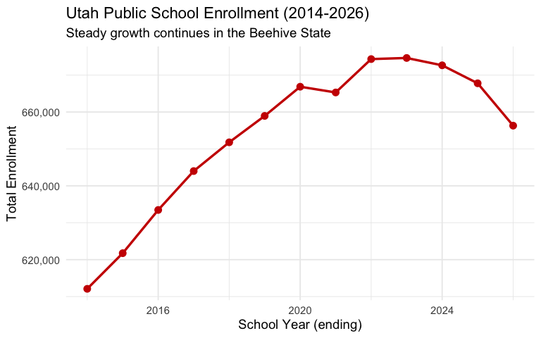
1. Utah’s enrollment continues to grow
Utah has one of the youngest populations in the nation and continues to see steady enrollment growth, unlike many states that saw declines after COVID.
enr <- fetch_enr_multi(available_years, use_cache = TRUE)

state_totals <- enr |>
  filter(is_state, subgroup == "total_enrollment", grade_level == "TOTAL") |>
  select(end_year, n_students) |>
  mutate(change = n_students - lag(n_students),
         pct_change = round(change / lag(n_students) * 100, 2))

state_totals
#>    end_year n_students change pct_change
#> 1      2014     612088     NA         NA
#> 2      2015     621748   9660       1.58
#> 3      2016     633461  11713       1.88
#> 4      2017     644004  10543       1.66
#> 5      2018     651796   7792       1.21
#> 6      2019     658952   7156       1.10
#> 7      2020     666858   7906       1.20
#> 8      2021     665306  -1552      -0.23
#> 9      2022     674351   9045       1.36
#> 10     2023     674650    299       0.04
#> 11     2024     672662  -1988      -0.29
#> 12     2025     667789  -4873      -0.72
#> 13     2026     656310 -11479      -1.72
ggplot(state_totals, aes(x = end_year, y = n_students)) +
  geom_line(linewidth = 1.2, color = "#CC0000") +
  geom_point(size = 3, color = "#CC0000") +
  scale_y_continuous(labels = scales::comma) +
  labs(
    title = paste0("Utah Public School Enrollment (", min_year, "-", max_year, ")"),
    subtitle = "Steady growth continues in the Beehive State",
    x = "School Year (ending)",
    y = "Total Enrollment"
  )
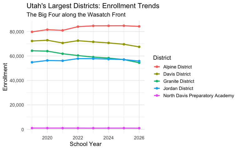
2. Granite and Alpine are Utah’s enrollment giants
Utah’s two largest districts–Granite and Alpine–each serve well over 60,000 students, but their trajectories differ. Salt Lake City has seen declines while suburban districts grow.
large_districts <- enr |>
  filter(is_district, subgroup == "total_enrollment", grade_level == "TOTAL",
         grepl("Granite|Alpine|Davis|Jordan|Canyons|Salt Lake City", district_name, ignore.case = TRUE)) |>
  select(end_year, district_name, n_students)

large_districts |>
  filter(end_year == max(end_year)) |>
  arrange(desc(n_students))
#>   end_year                   district_name n_students
#> 1     2026                 Alpine District      84215
#> 2     2026                  Davis District      67466
#> 3     2026                 Jordan District      55820
#> 4     2026                Granite District      54467
#> 5     2026                Canyons District      31499
#> 6     2026 North Davis Preparatory Academy        933
enr |>
  filter(is_district, subgroup == "total_enrollment", grade_level == "TOTAL",
         grepl("Granite|Alpine|Davis|Jordan", district_name, ignore.case = TRUE)) |>
  ggplot(aes(x = end_year, y = n_students, color = district_name)) +
  geom_line(linewidth = 1.2) +
  geom_point(size = 2) +
  scale_y_continuous(labels = scales::comma) +
  labs(
    title = "Utah's Largest Districts: Enrollment Trends",
    subtitle = "The Big Four along the Wasatch Front",
    x = "School Year",
    y = "Enrollment",
    color = "District"
  )
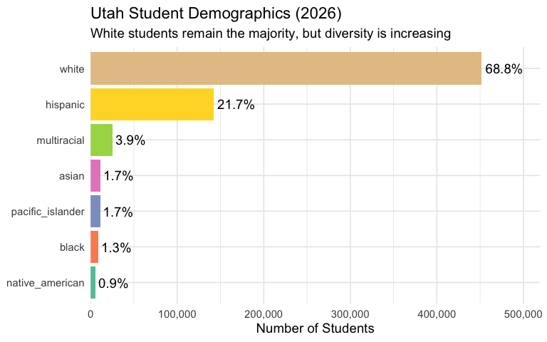
3. Utah’s student body is diversifying
While Utah remains less diverse than national averages, Hispanic enrollment has grown substantially over the past decade, now representing a significant share of students.
enr_latest <- fetch_enr(max_year, use_cache = TRUE)

demographics <- enr_latest |>
  filter(is_state, grade_level == "TOTAL",
         subgroup %in% c("hispanic", "white", "black", "asian", "native_american", "pacific_islander", "multiracial")) |>
  mutate(pct = round(pct * 100, 1)) |>
  select(subgroup, n_students, pct) |>
  arrange(desc(n_students))

demographics
#>           subgroup n_students  pct
#> 1            white     451812 68.8
#> 2         hispanic     142284 21.7
#> 3      multiracial      25385  3.9
#> 4            asian      11385  1.7
#> 5 pacific_islander      10973  1.7
#> 6            black       8806  1.3
#> 7  native_american       5665  0.9
demographics |>
  mutate(subgroup = forcats::fct_reorder(subgroup, n_students)) |>
  ggplot(aes(x = n_students, y = subgroup, fill = subgroup)) +
  geom_col(show.legend = FALSE) +
  geom_text(aes(label = paste0(pct, "%")), hjust = -0.1) +
  scale_x_continuous(labels = scales::comma, expand = expansion(mult = c(0, 0.15))) +
  scale_fill_brewer(palette = "Set2") +
  labs(
    title = paste0("Utah Student Demographics (", max_year, ")"),
    subtitle = "White students remain the majority, but diversity is increasing",
    x = "Number of Students",
    y = NULL
  )
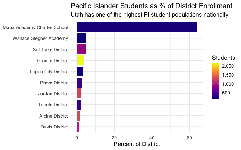
4. Pacific Islander students are a unique Utah story
Utah has one of the highest concentrations of Pacific Islander students in the nation, reflecting the state’s significant Polynesian community, particularly in Salt Lake County.
pi_districts <- enr_latest |>
  filter(is_district, grade_level == "TOTAL", subgroup == "pacific_islander") |>
  filter(n_students > 100) |>
  mutate(pct = round(pct * 100, 2)) |>
  select(district_name, n_students, pct) |>
  arrange(desc(pct)) |>
  head(10)

pi_districts
#>                  district_name n_students   pct
#> 1  Mana Academy Charter School        193 64.12
#> 2      Wallace Stegner Academy        145  5.09
#> 3           Salt Lake District        886  5.02
#> 4             Granite District       2146  3.94
#> 5          Logan City District        160  3.15
#> 6               Provo District        388  2.98
#> 7              Jordan District       1275  2.28
#> 8              Tooele District        340  2.16
#> 9              Alpine District       1331  1.58
#> 10              Davis District       1023  1.52
pi_districts |>
  mutate(district_name = forcats::fct_reorder(district_name, pct)) |>
  ggplot(aes(x = pct, y = district_name, fill = n_students)) +
  geom_col() +
  scale_fill_viridis_c(option = "plasma", labels = scales::comma) +
  labs(
    title = "Pacific Islander Students as % of District Enrollment",
    subtitle = "Utah has one of the highest PI student populations nationally",
    x = "Percent of District",
    y = NULL,
    fill = "Students"
  )
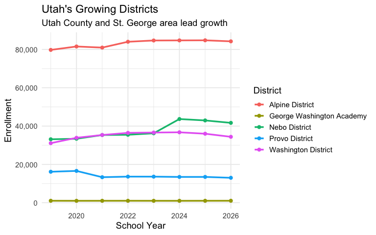
5. Utah County is the growth engine
Provo, Alpine, and Nebo districts in Utah County are seeing consistent growth as young families settle along the I-15 corridor south of Salt Lake.
utah_county <- enr |>
  filter(is_district, subgroup == "total_enrollment", grade_level == "TOTAL",
         grepl("Alpine|Provo|Nebo", district_name, ignore.case = TRUE)) |>
  group_by(district_name) |>
  arrange(end_year) |>
  summarize(
    first_year = first(n_students),
    last_year = last(n_students),
    pct_change = round((last_year / first_year - 1) * 100, 1),
    .groups = "drop"
  ) |>
  arrange(desc(pct_change))

stopifnot(nrow(utah_county) > 0)
utah_county
#> # A tibble: 3 × 4
#>   district_name   first_year last_year pct_change
#>   <chr>                <dbl>     <dbl>      <dbl>
#> 1 Nebo District        33117     41675       25.8
#> 2 Alpine District      79748     84215        5.6
#> 3 Provo District       16165     13010      -19.5
enr |>
  filter(is_district, subgroup == "total_enrollment", grade_level == "TOTAL",
         grepl("Alpine|Provo|Nebo|Washington", district_name, ignore.case = TRUE)) |>
  ggplot(aes(x = end_year, y = n_students, color = district_name)) +
  geom_line(linewidth = 1.2) +
  geom_point(size = 2) +
  scale_y_continuous(labels = scales::comma) +
  labs(
    title = "Utah's Growing Districts",
    subtitle = "Utah County and St. George area lead growth",
    x = "School Year",
    y = "Enrollment",
    color = "District"
  )
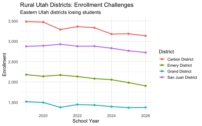
6. Rural districts face decline
While the Wasatch Front booms, rural districts in southern and eastern Utah face enrollment pressure as families move to urban centers for jobs and services.
rural <- enr |>
  filter(is_district, subgroup == "total_enrollment", grade_level == "TOTAL",
         grepl("Carbon|Emery|Grand|San Juan|Millard", district_name, ignore.case = TRUE)) |>
  group_by(district_name) |>
  filter(n() >= 5) |>
  arrange(end_year) |>
  summarize(
    first_year = first(n_students),
    last_year = last(n_students),
    pct_change = round((last_year / first_year - 1) * 100, 1),
    .groups = "drop"
  ) |>
  arrange(pct_change)

stopifnot(nrow(rural) > 0)
rural
#> # A tibble: 5 × 4
#>   district_name     first_year last_year pct_change
#>   <chr>                  <dbl>     <dbl>      <dbl>
#> 1 Emery District          2181      1907      -12.6
#> 2 Carbon District         3484      3135      -10
#> 3 Grand District          1520      1376       -9.5
#> 4 San Juan District       2876      2725       -5.3
#> 5 Millard District        2916      2997        2.8
enr |>
  filter(is_district, subgroup == "total_enrollment", grade_level == "TOTAL",
         grepl("Carbon|Emery|Grand|San Juan", district_name, ignore.case = TRUE)) |>
  ggplot(aes(x = end_year, y = n_students, color = district_name)) +
  geom_line(linewidth = 1.2) +
  geom_point(size = 2) +
  scale_y_continuous(labels = scales::comma) +
  labs(
    title = "Rural Utah Districts: Enrollment Challenges",
    subtitle = "Eastern Utah districts losing students",
    x = "School Year",
    y = "Enrollment",
    color = "District"
  )
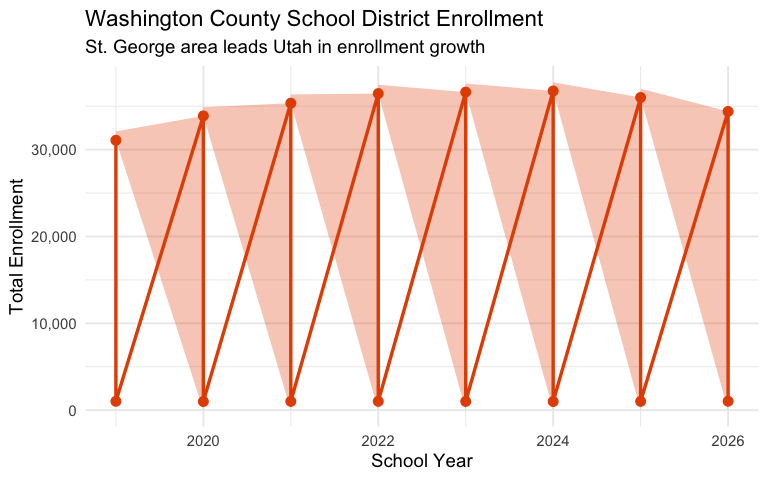
7. Washington County is Utah’s fastest-growing region
The St. George area (Washington County School District) has exploded with growth as retirees and remote workers flock to southern Utah.
washington <- enr |>
  filter(is_district, subgroup == "total_enrollment", grade_level == "TOTAL",
         grepl("Washington", district_name, ignore.case = TRUE)) |>
  select(end_year, district_name, n_students) |>
  mutate(change = n_students - lag(n_students),
         pct_change = round(change / lag(n_students) * 100, 1))

washington
#>    end_year             district_name n_students change pct_change
#> 1      2019       Washington District      31074     NA         NA
#> 2      2019 George Washington Academy       1021 -30053      -96.7
#> 3      2020       Washington District      33884  32863     3218.7
#> 4      2020 George Washington Academy        998 -32886      -97.1
#> 5      2021       Washington District      35346  34348     3441.7
#> 6      2021 George Washington Academy       1011 -34335      -97.1
#> 7      2022       Washington District      36453  35442     3505.6
#> 8      2022 George Washington Academy       1017 -35436      -97.2
#> 9      2023       Washington District      36623  35606     3501.1
#> 10     2023 George Washington Academy       1003 -35620      -97.3
#> 11     2024       Washington District      36753  35750     3564.3
#> 12     2024 George Washington Academy        996 -35757      -97.3
#> 13     2025       Washington District      36006  35010     3515.1
#> 14     2025 George Washington Academy       1014 -34992      -97.2
#> 15     2026       Washington District      34396  33382     3292.1
#> 16     2026 George Washington Academy       1030 -33366      -97.0
washington |>
  ggplot(aes(x = end_year, y = n_students)) +
  geom_area(fill = "#E65100", alpha = 0.3) +
  geom_line(color = "#E65100", linewidth = 1.2) +
  geom_point(color = "#E65100", size = 3) +
  scale_y_continuous(labels = scales::comma) +
  labs(
    title = "Washington County School District Enrollment",
    subtitle = "St. George area leads Utah in enrollment growth",
    x = "School Year",
    y = "Total Enrollment"
  )
8. Charter schools serve a growing share of Utah students
Utah has a robust charter school sector, with dozens of charter schools across the state serving students who seek alternatives to traditional district schools.
state_total <- enr_latest |>
  filter(is_state, subgroup == "total_enrollment", grade_level == "TOTAL") |>
  pull(n_students)

charter_total <- enr_latest |>
  filter(is_charter, subgroup == "total_enrollment", grade_level == "TOTAL") |>
  summarize(charter_total = sum(n_students, na.rm = TRUE)) |>
  pull(charter_total)

charter_summary <- tibble(
  sector = c("All Public Schools", "Charter Schools"),
  enrollment = c(state_total, charter_total),
  pct = c(100, round(charter_total / state_total * 100, 1))
)

charter_summary
#> # A tibble: 2 × 3
#>   sector             enrollment   pct
#>   <chr>                   <dbl> <dbl>
#> 1 All Public Schools     656310   100
#> 2 Charter Schools        170536    26
tibble(
  sector = c("Traditional Districts", "Charter Schools"),
  enrollment = c(state_total - charter_total, charter_total)
) |>
  mutate(pct = enrollment / sum(enrollment) * 100,
         label = paste0(round(pct, 1), "%")) |>
  ggplot(aes(x = "", y = enrollment, fill = sector)) +
  geom_col(width = 1) +
  coord_polar(theta = "y") +
  geom_text(aes(label = label), position = position_stack(vjust = 0.5), color = "white", size = 5) +
  scale_fill_manual(values = c("Traditional Districts" = "#1976D2", "Charter Schools" = "#43A047")) +
  labs(
    title = paste0("Utah Public School Enrollment by Sector (", max_year, ")"),
    subtitle = "Charter schools serve a growing share of students",
    fill = NULL
  ) +
  theme_void() +
  theme(legend.position = "bottom", plot.title = element_text(hjust = 0.5), plot.subtitle = element_text(hjust = 0.5))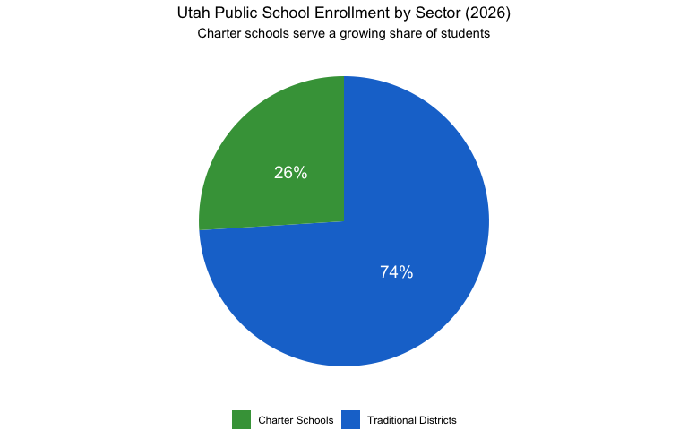
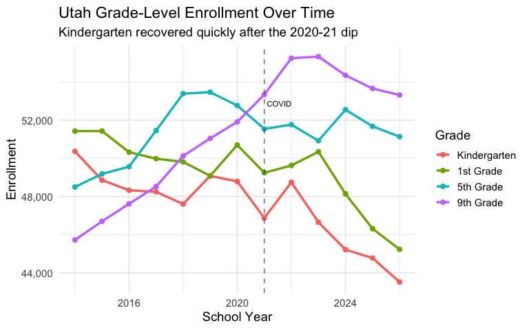
9. Kindergarten enrollment dipped during COVID but recovered
Unlike many states, Utah saw kindergarten enrollment bounce back relatively quickly after COVID disruptions.
covid_grades <- enr |>
  filter(is_state, subgroup == "total_enrollment",
         grade_level %in% c("K", "01", "05", "09")) |>
  select(end_year, grade_level, n_students) |>
  pivot_wider(names_from = grade_level, values_from = n_students)

covid_grades
#> # A tibble: 13 × 5
#>    end_year     K  `01`  `05`  `09`
#>       <int> <dbl> <dbl> <dbl> <dbl>
#>  1     2014 50363 51424 48499 45721
#>  2     2015 48859 51431 49181 46699
#>  3     2016 48327 50322 49563 47616
#>  4     2017 48242 49981 51455 48522
#>  5     2018 47605 49812 53389 50125
#>  6     2019 49081 49081 53465 51044
#>  7     2020 48789 50699 52766 51908
#>  8     2021 46874 49242 51542 53340
#>  9     2022 48744 49624 51764 55245
#> 10     2023 46655 50346 50921 55330
#> 11     2024 45217 48138 52547 54351
#> 12     2025 44776 46313 51677 53658
#> 13     2026 43519 45232 51133 53318
enr |>
  filter(is_state, subgroup == "total_enrollment",
         grade_level %in% c("K", "01", "05", "09")) |>
  mutate(grade_level = factor(grade_level, levels = c("K", "01", "05", "09"),
                               labels = c("Kindergarten", "1st Grade", "5th Grade", "9th Grade"))) |>
  ggplot(aes(x = end_year, y = n_students, color = grade_level)) +
  geom_line(linewidth = 1.2) +
  geom_point(size = 2) +
  geom_vline(xintercept = 2021, linetype = "dashed", alpha = 0.5) +
  annotate("text", x = 2021, y = max(covid_grades$K) * 1.05, label = "COVID", hjust = -0.1, size = 3) +
  scale_y_continuous(labels = scales::comma) +
  labs(
    title = "Utah Grade-Level Enrollment Over Time",
    subtitle = "Kindergarten recovered quickly after the 2020-21 dip",
    x = "School Year",
    y = "Enrollment",
    color = "Grade"
  )
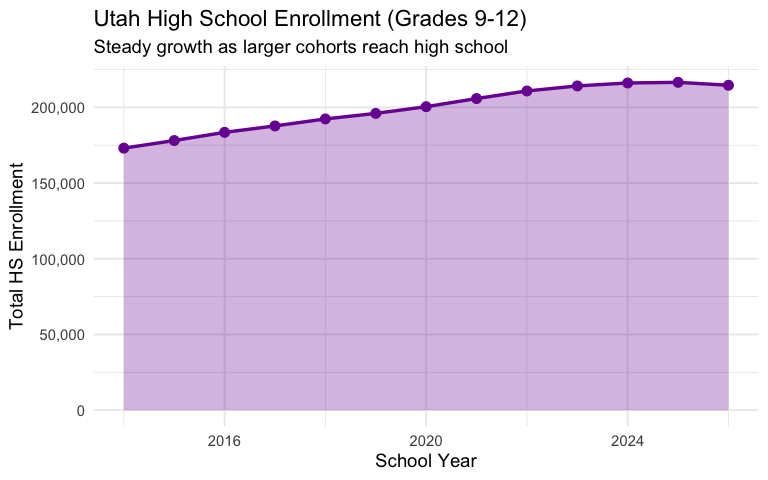
10. High school enrollment is surging
As larger elementary cohorts from the 2010s move through the system, Utah high schools are seeing significant enrollment growth.
hs_trend <- enr |>
  filter(is_state, subgroup == "total_enrollment",
         grade_level %in% c("09", "10", "11", "12")) |>
  group_by(end_year) |>
  summarize(hs_total = sum(n_students, na.rm = TRUE), .groups = "drop") |>
  mutate(change = hs_total - lag(hs_total),
         pct_change = round(change / lag(hs_total) * 100, 1))

hs_trend
#> # A tibble: 13 × 4
#>    end_year hs_total change pct_change
#>       <int>    <dbl>  <dbl>      <dbl>
#>  1     2014   173049     NA       NA
#>  2     2015   178071   5022        2.9
#>  3     2016   183492   5421        3
#>  4     2017   187727   4235        2.3
#>  5     2018   192340   4613        2.5
#>  6     2019   196008   3668        1.9
#>  7     2020   200437   4429        2.3
#>  8     2021   205808   5371        2.7
#>  9     2022   210817   5009        2.4
#> 10     2023   214148   3331        1.6
#> 11     2024   216094   1946        0.9
#> 12     2025   216526    432        0.2
#> 13     2026   214601  -1925       -0.9
hs_trend |>
  ggplot(aes(x = end_year, y = hs_total)) +
  geom_area(fill = "#7B1FA2", alpha = 0.3) +
  geom_line(color = "#7B1FA2", linewidth = 1.2) +
  geom_point(color = "#7B1FA2", size = 3) +
  scale_y_continuous(labels = scales::comma) +
  labs(
    title = "Utah High School Enrollment (Grades 9-12)",
    subtitle = "Steady growth as larger cohorts reach high school",
    x = "School Year",
    y = "Total HS Enrollment"
  )
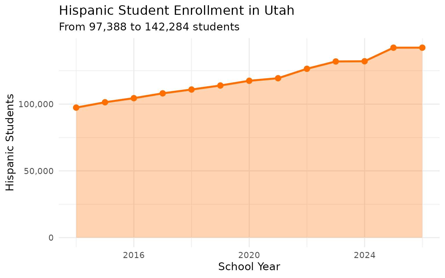
11. Hispanic enrollment grew 46% since 2014
Utah’s Hispanic student population has grown significantly faster than overall enrollment, adding nearly 45,000 students in just over a decade.
hispanic <- enr |>
  filter(is_state, grade_level == "TOTAL", subgroup == "hispanic") |>
  select(end_year, n_students) |>
  mutate(change = n_students - lag(n_students),
         pct_change = round(change / lag(n_students) * 100, 1))

hispanic
#>    end_year n_students change pct_change
#> 1      2014      97388     NA         NA
#> 2      2015     101390   4002        4.1
#> 3      2016     104457   3067        3.0
#> 4      2017     108074   3617        3.5
#> 5      2018     110931   2857        2.6
#> 6      2019     113945   3014        2.7
#> 7      2020     117486   3541        3.1
#> 8      2021     119393   1907        1.6
#> 9      2022     126467   7074        5.9
#> 10     2023     131954   5487        4.3
#> 11     2024     132110    156        0.1
#> 12     2025     142267  10157        7.7
#> 13     2026     142284     17        0.0
hispanic |>
  ggplot(aes(x = end_year, y = n_students)) +
  geom_area(fill = "#FF6F00", alpha = 0.3) +
  geom_line(color = "#FF6F00", linewidth = 1.2) +
  geom_point(color = "#FF6F00", size = 3) +
  scale_y_continuous(labels = scales::comma) +
  labs(
    title = "Hispanic Student Enrollment in Utah",
    subtitle = paste0("From ", format(min(hispanic$n_students), big.mark = ","), " to ",
                      format(max(hispanic$n_students), big.mark = ","), " students"),
    x = "School Year",
    y = "Hispanic Students"
  )
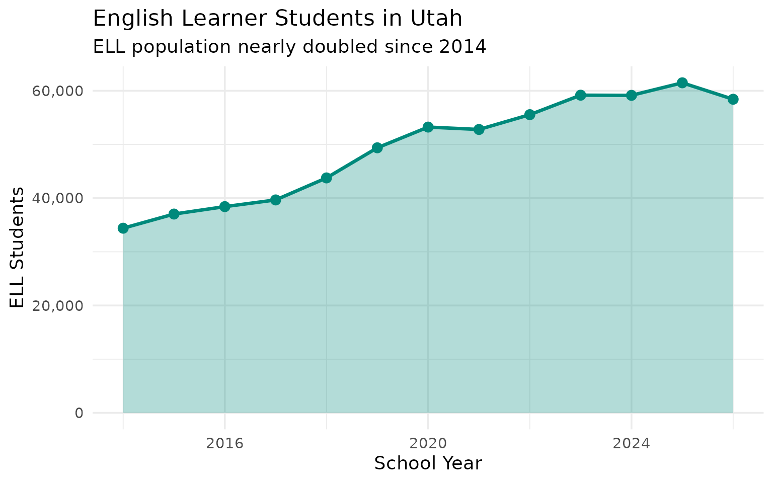
12. English learner population nearly doubled
The number of English learners (ELL/LEP) in Utah schools has grown from 34,000 to over 61,000 since 2014–an 79% increase.
ell_trend <- enr |>
  filter(is_state, grade_level == "TOTAL", subgroup == "lep") |>
  select(end_year, n_students, pct) |>
  mutate(pct = round(pct * 100, 1),
         change = n_students - lag(n_students),
         pct_change = round(change / lag(n_students) * 100, 1))

ell_trend
#>    end_year n_students pct change pct_change
#> 1      2014      34394 5.6     NA         NA
#> 2      2015      37033 6.0   2639        7.7
#> 3      2016      38414 6.1   1381        3.7
#> 4      2017      39662 6.2   1248        3.2
#> 5      2018      43763 6.7   4101       10.3
#> 6      2019      49374 7.5   5611       12.8
#> 7      2020      53234 8.0   3860        7.8
#> 8      2021      52788 7.9   -446       -0.8
#> 9      2022      55546 8.2   2758        5.2
#> 10     2023      59176 8.8   3630        6.5
#> 11     2024      59147 8.8    -29        0.0
#> 12     2025      61481 9.2   2334        3.9
#> 13     2026      58419 8.9  -3062       -5.0
ell_trend |>
  ggplot(aes(x = end_year, y = n_students)) +
  geom_area(fill = "#00897B", alpha = 0.3) +
  geom_line(color = "#00897B", linewidth = 1.2) +
  geom_point(color = "#00897B", size = 3) +
  scale_y_continuous(labels = scales::comma) +
  labs(
    title = "English Learner Students in Utah",
    subtitle = "ELL population nearly doubled since 2014",
    x = "School Year",
    y = "ELL Students"
  )
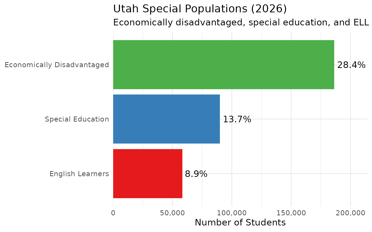
13. Nearly 1 in 3 students are economically disadvantaged
About 29% of Utah students qualify as economically disadvantaged–lower than the national average but still representing nearly 194,000 students.
special_pops <- enr_latest |>
  filter(is_state, grade_level == "TOTAL",
         subgroup %in% c("econ_disadv", "lep", "special_ed")) |>
  mutate(pct = round(pct * 100, 1)) |>
  select(subgroup, n_students, pct) |>
  arrange(desc(n_students))

special_pops
#>      subgroup n_students  pct
#> 1 econ_disadv     186361 28.4
#> 2  special_ed      89893 13.7
#> 3         lep      58419  8.9
special_pops |>
  mutate(subgroup = forcats::fct_recode(subgroup,
    "Economically Disadvantaged" = "econ_disadv",
    "Special Education" = "special_ed",
    "English Learners" = "lep")) |>
  mutate(subgroup = forcats::fct_reorder(subgroup, n_students)) |>
  ggplot(aes(x = n_students, y = subgroup, fill = subgroup)) +
  geom_col(show.legend = FALSE) +
  geom_text(aes(label = paste0(pct, "%")), hjust = -0.1) +
  scale_x_continuous(labels = scales::comma, expand = expansion(mult = c(0, 0.15))) +
  scale_fill_brewer(palette = "Set1") +
  labs(
    title = paste0("Utah Special Populations (", max_year, ")"),
    subtitle = "Economically disadvantaged, special education, and ELL students",
    x = "Number of Students",
    y = NULL
  )
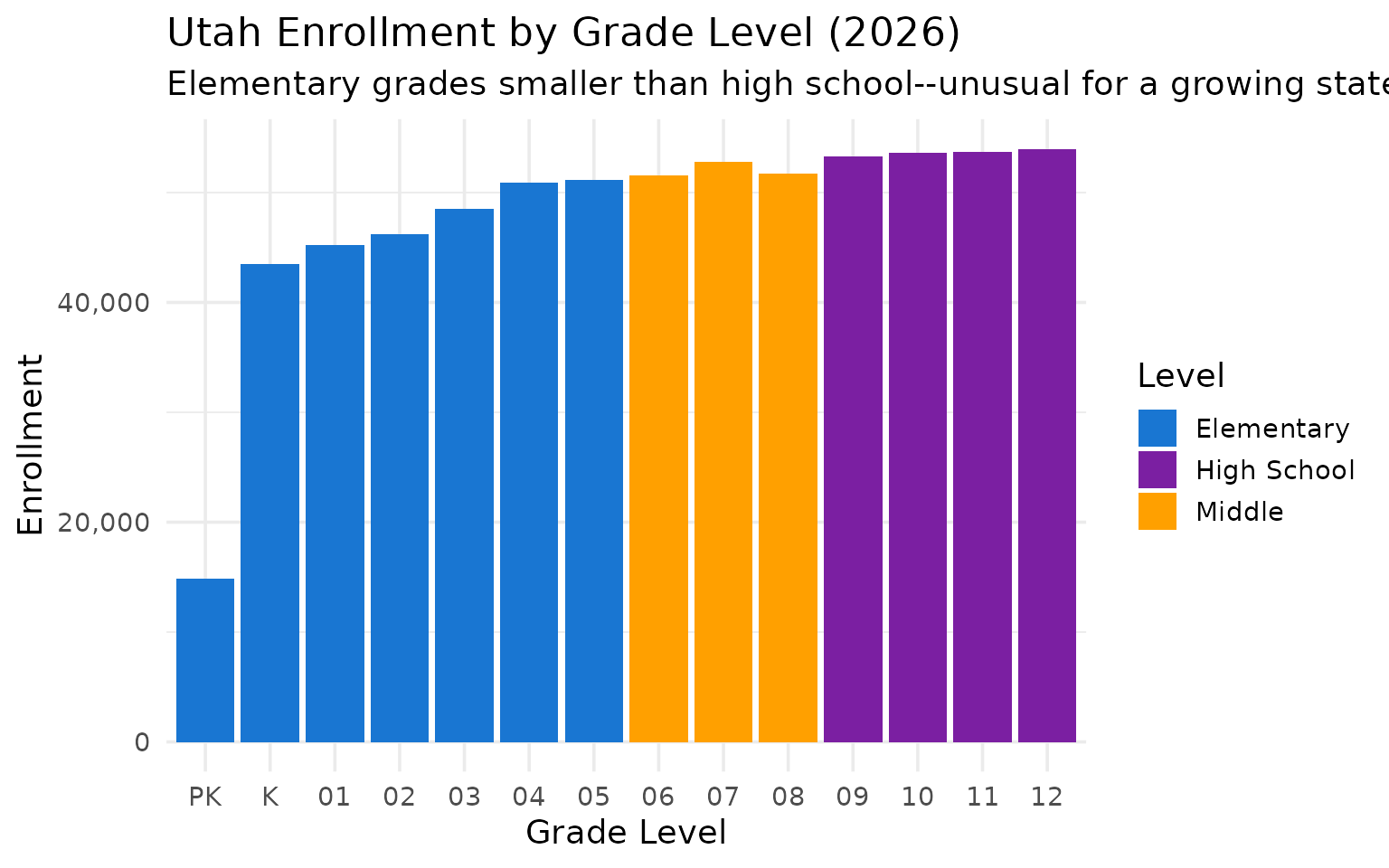
14. Elementary enrollment is declining while high school grows
Utah kindergarten enrollment dropped 11% since its 2014 peak, even as high school grades are at record levels. This points to future enrollment declines.
grades <- enr_latest |>
  filter(is_state, subgroup == "total_enrollment") |>
  filter(!grade_level %in% c("TOTAL")) |>
  select(grade_level, n_students) |>
  arrange(desc(n_students))

grades
#>    grade_level n_students
#> 1           12      53982
#> 2           11      53721
#> 3           10      53580
#> 4           09      53318
#> 5           07      52826
#> 6           08      51752
#> 7           06      51547
#> 8           05      51133
#> 9           04      50931
#> 10          03      48524
#> 11          02      46245
#> 12          01      45232
#> 13           K      43519
#> 14          PK      14869
grades |>
  mutate(grade_level = factor(grade_level,
         levels = c("PK", "K", "01", "02", "03", "04", "05", "06", "07", "08", "09", "10", "11", "12"))) |>
  mutate(level = case_when(
    grade_level %in% c("PK", "K", "01", "02", "03", "04", "05") ~ "Elementary",
    grade_level %in% c("06", "07", "08") ~ "Middle",
    TRUE ~ "High School"
  )) |>
  ggplot(aes(x = grade_level, y = n_students, fill = level)) +
  geom_col() +
  scale_y_continuous(labels = scales::comma) +
  scale_fill_manual(values = c("Elementary" = "#1976D2", "Middle" = "#FFA000", "High School" = "#7B1FA2")) +
  labs(
    title = paste0("Utah Enrollment by Grade Level (", max_year, ")"),
    subtitle = "Elementary grades smaller than high school--unusual for a growing state",
    x = "Grade Level",
    y = "Enrollment",
    fill = "Level"
  )
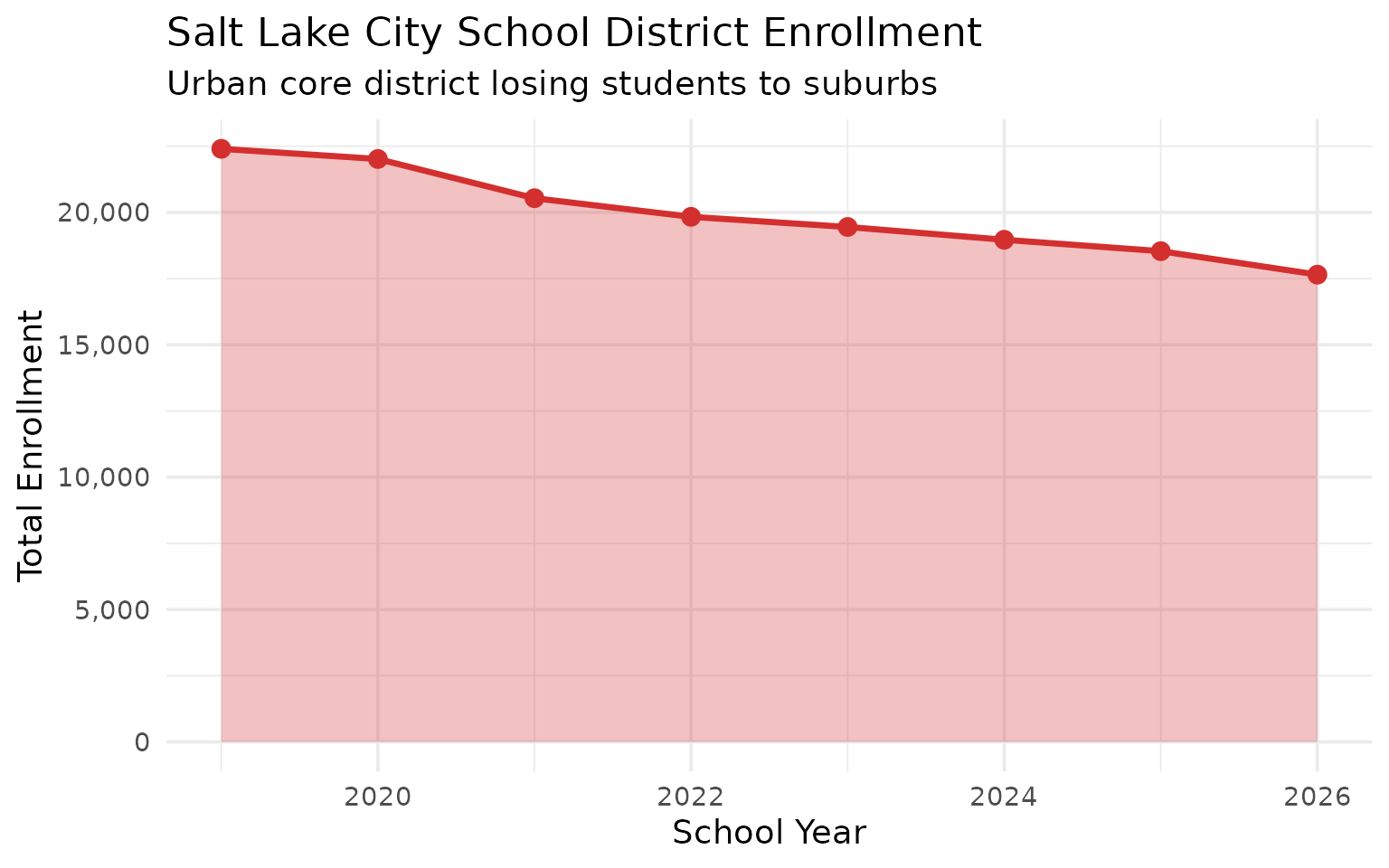
15. Salt Lake City district lost 17% of students since 2019
While suburban districts boom, Salt Lake City School District has declined from over 22,000 to under 19,000 students–a loss driven by housing costs and demographic shifts in the urban core.
salt_lake <- enr |>
  filter(is_district, subgroup == "total_enrollment", grade_level == "TOTAL",
         district_name == "Salt Lake District") |>
  select(end_year, district_name, n_students) |>
  mutate(change = n_students - lag(n_students),
         pct_change = round(change / lag(n_students) * 100, 1))

salt_lake
#>   end_year      district_name n_students change pct_change
#> 1     2019 Salt Lake District      22401     NA         NA
#> 2     2020 Salt Lake District      22017   -384       -1.7
#> 3     2021 Salt Lake District      20536  -1481       -6.7
#> 4     2022 Salt Lake District      19833   -703       -3.4
#> 5     2023 Salt Lake District      19449   -384       -1.9
#> 6     2024 Salt Lake District      18966   -483       -2.5
#> 7     2025 Salt Lake District      18535   -431       -2.3
#> 8     2026 Salt Lake District      17649   -886       -4.8
salt_lake |>
  ggplot(aes(x = end_year, y = n_students)) +
  geom_area(fill = "#D32F2F", alpha = 0.3) +
  geom_line(color = "#D32F2F", linewidth = 1.2) +
  geom_point(color = "#D32F2F", size = 3) +
  scale_y_continuous(labels = scales::comma) +
  labs(
    title = "Salt Lake City School District Enrollment",
    subtitle = "Urban core district losing students to suburbs",
    x = "School Year",
    y = "Total Enrollment"
  )
Summary
Utah’s school enrollment data reveals:
- Continued growth: Unlike many states, Utah continues to add students
- Wasatch Front dominance: The Salt Lake-Provo corridor holds most students
- Southern boom: Washington County (St. George) is the fastest-growing region
- Rural challenges: Eastern Utah districts losing students to urban areas
- Diversifying demographics: Hispanic and Pacific Islander populations growing
- Charter expansion: Charter schools serve a meaningful share of students
These patterns reflect Utah’s unique demographics–the youngest state in the nation–and rapid population growth along the Wasatch Front and in southwestern Utah.
Data sourced from the Utah State Board of Education Data and Statistics.
Session Info
sessionInfo()
#> R version 4.5.2 (2025-10-31)
#> Platform: x86_64-pc-linux-gnu
#> Running under: Ubuntu 24.04.3 LTS
#>
#> Matrix products: default
#> BLAS:   /usr/lib/x86_64-linux-gnu/openblas-pthread/libblas.so.3
#> LAPACK: /usr/lib/x86_64-linux-gnu/openblas-pthread/libopenblasp-r0.3.26.so;  LAPACK version 3.12.0
#>
#> locale:
#>  [1] LC_CTYPE=C.UTF-8       LC_NUMERIC=C           LC_TIME=C.UTF-8
#>  [4] LC_COLLATE=C.UTF-8     LC_MONETARY=C.UTF-8    LC_MESSAGES=C.UTF-8
#>  [7] LC_PAPER=C.UTF-8       LC_NAME=C              LC_ADDRESS=C
#> [10] LC_TELEPHONE=C         LC_MEASUREMENT=C.UTF-8 LC_IDENTIFICATION=C
#>
#> time zone: UTC
#> tzcode source: system (glibc)
#>
#> attached base packages:
#> [1] stats     graphics  grDevices utils     datasets  methods   base
#>
#> other attached packages:
#> [1] ggplot2_4.0.2      tidyr_1.3.2        dplyr_1.2.0        utschooldata_0.1.0
#>
#> loaded via a namespace (and not attached):
#>  [1] gtable_0.3.6       jsonlite_2.0.0     compiler_4.5.2     tidyselect_1.2.1
#>  [5] jquerylib_0.1.4    systemfonts_1.3.2  scales_1.4.0       textshaping_1.0.5
#>  [9] readxl_1.4.5       yaml_2.3.12        fastmap_1.2.0      R6_2.6.1
#> [13] labeling_0.4.3     generics_0.1.4     curl_7.0.0         knitr_1.51
#> [17] forcats_1.0.1      tibble_3.3.1       desc_1.4.3         bslib_0.10.0
#> [21] pillar_1.11.1      RColorBrewer_1.1-3 rlang_1.1.7        utf8_1.2.6
#> [25] cachem_1.1.0       xfun_0.56          fs_1.6.7           sass_0.4.10
#> [29] S7_0.2.1           viridisLite_0.4.3  cli_3.6.5          withr_3.0.2
#> [33] pkgdown_2.2.0      magrittr_2.0.4     digest_0.6.39      grid_4.5.2
#> [37] rappdirs_0.3.4     lifecycle_1.0.5    vctrs_0.7.1        evaluate_1.0.5
#> [41] glue_1.8.0         cellranger_1.1.0   farver_2.1.2       codetools_0.2-20
#> [45] ragg_1.5.1         httr_1.4.8         rmarkdown_2.30     purrr_1.2.1
#> [49] tools_4.5.2        pkgconfig_2.0.3    htmltools_0.5.9