15 Insights from Washington School Enrollment Data
Source:vignettes/enrollment_hooks.Rmd
enrollment_hooks.Rmd
library(waschooldata)
library(dplyr)
library(tidyr)
library(ggplot2)

theme_set(theme_minimal(base_size = 14))
This vignette explores Washington’s public school enrollment data, surfacing key trends across 16 years of data (2010-2025).
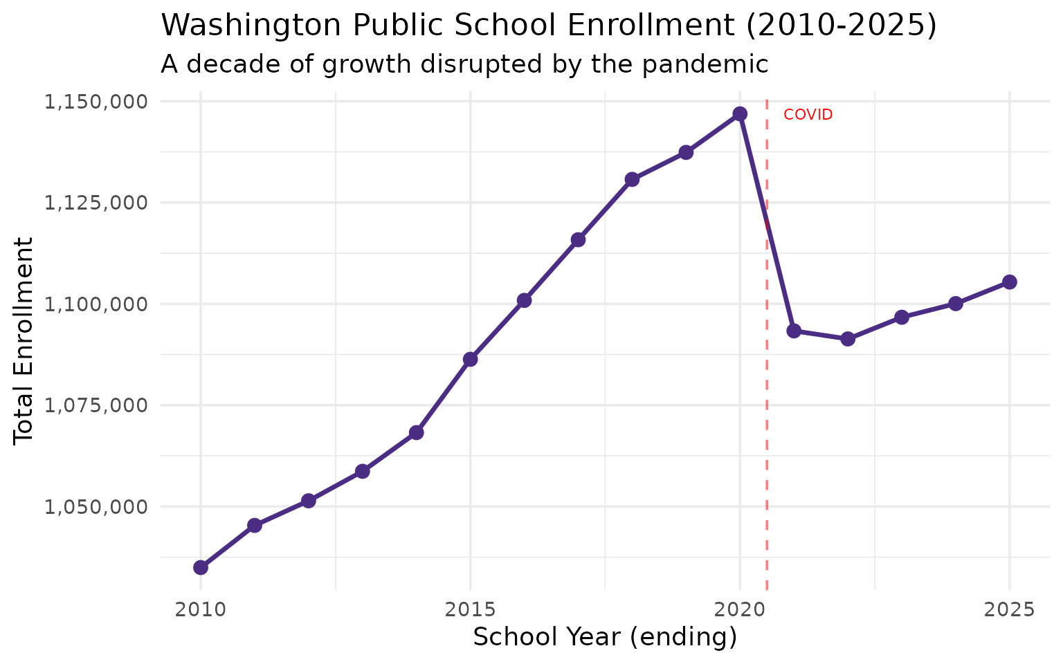
1. Washington added 70,000 students over 16 years before COVID reversed the trend
The Evergreen State grew enrollment steadily from 1.03 million to nearly 1.15 million before the pandemic wiped out years of gains.
enr <- fetch_enr_multi(2010:2025, use_cache = TRUE)

state_totals <- enr |>
  filter(is_state, subgroup == "total_enrollment", grade_level == "TOTAL") |>
  select(end_year, n_students) |>
  mutate(change = n_students - lag(n_students),
         pct_change = round(change / lag(n_students) * 100, 2))
stopifnot(nrow(state_totals) > 0)

state_totals
#>    end_year n_students change pct_change
#> 1      2010    1034935     NA         NA
#> 2      2011    1045333  10398       1.00
#> 3      2012    1051404   6071       0.58
#> 4      2013    1058680   7276       0.69
#> 5      2014    1068234   9554       0.90
#> 6      2015    1086314  18080       1.69
#> 7      2016    1100849  14535       1.34
#> 8      2017    1115820  14971       1.36
#> 9      2018    1130714  14894       1.33
#> 10     2019    1137367   6653       0.59
#> 11     2020    1146882   9515       0.84
#> 12     2021    1093331 -53551      -4.67
#> 13     2022    1091343  -1988      -0.18
#> 14     2023    1096695   5352       0.49
#> 15     2024    1100059   3364       0.31
#> 16     2025    1105384   5325       0.48
print(state_totals)
#>    end_year n_students change pct_change
#> 1      2010    1034935     NA         NA
#> 2      2011    1045333  10398       1.00
#> 3      2012    1051404   6071       0.58
#> 4      2013    1058680   7276       0.69
#> 5      2014    1068234   9554       0.90
#> 6      2015    1086314  18080       1.69
#> 7      2016    1100849  14535       1.34
#> 8      2017    1115820  14971       1.36
#> 9      2018    1130714  14894       1.33
#> 10     2019    1137367   6653       0.59
#> 11     2020    1146882   9515       0.84
#> 12     2021    1093331 -53551      -4.67
#> 13     2022    1091343  -1988      -0.18
#> 14     2023    1096695   5352       0.49
#> 15     2024    1100059   3364       0.31
#> 16     2025    1105384   5325       0.48

ggplot(state_totals, aes(x = end_year, y = n_students)) +
  geom_line(linewidth = 1.2, color = "#4B2E83") +
  geom_point(size = 3, color = "#4B2E83") +
  geom_vline(xintercept = 2020.5, linetype = "dashed", color = "red", alpha = 0.5) +
  annotate("text", x = 2020.8, y = max(state_totals$n_students, na.rm = TRUE),
           label = "COVID", hjust = 0, color = "red", size = 3) +
  scale_y_continuous(labels = scales::comma) +
  labs(
    title = "Washington Public School Enrollment (2010-2025)",
    subtitle = "A decade of growth disrupted by the pandemic",
    x = "School Year (ending)",
    y = "Total Enrollment"
  )
2. Seattle peaked at 56,000 students then lost 9% in five years
Washington’s largest district peaked in 2020 and has lost nearly 5,000 students since, even as tech industry growth transformed the region.
seattle <- enr |>
  filter(is_district, subgroup == "total_enrollment", grade_level == "TOTAL",
         grepl("Seattle", district_name, ignore.case = TRUE)) |>
  select(end_year, district_name, n_students) |>
  mutate(pct_of_peak = round(n_students / max(n_students) * 100, 1))
stopifnot(nrow(seattle) > 0)

seattle
#>    end_year                 district_name n_students pct_of_peak
#> 1      2010 Seattle School District No. 1      47058        84.0
#> 2      2011 Seattle School District No. 1      48299        86.2
#> 3      2012 Seattle School District No. 1      49851        88.9
#> 4      2013 Seattle School District No. 1      51201        91.3
#> 5      2014 Seattle School District No. 1      52181        93.1
#> 6      2015 Seattle School District No. 1      53361        95.2
#> 7      2016 Seattle School District No. 1      53767        95.9
#> 8      2017 Seattle School District No. 1      54722        97.6
#> 9      2018 Seattle School District No. 1      55321        98.7
#> 10     2019 Seattle School District No. 1      55325        98.7
#> 11     2020 Seattle School District No. 1      56051       100.0
#> 12     2021 Seattle School District No. 1      54021        96.4
#> 13     2022 Seattle School District No. 1      51653        92.2
#> 14     2023 Seattle School District No. 1      51528        91.9
#> 15     2024 Seattle School District No. 1      50968        90.9
#> 16     2025 Seattle School District No. 1      51200        91.3
top_districts <- enr |>
  filter(is_district, subgroup == "total_enrollment", grade_level == "TOTAL",
         end_year == 2025) |>
  arrange(desc(n_students)) |>
  head(5) |>
  pull(district_id)
stopifnot(length(top_districts) > 0)

top5_data <- enr |>
  filter(is_district, subgroup == "total_enrollment", grade_level == "TOTAL",
         district_id %in% top_districts)
stopifnot(nrow(top5_data) > 0)

print(top5_data |> filter(end_year == 2025) |> select(district_name, n_students))
#>                     district_name n_students
#> 1         Spokane School District      29690
#> 2 Lake Washington School District      31146
#> 3            Kent School District      25455
#> 4          Tacoma School District      29014
#> 5   Seattle School District No. 1      51200

ggplot(top5_data, aes(x = end_year, y = n_students, color = district_name)) +
  geom_line(linewidth = 1.2) +
  geom_point(size = 2) +
  geom_vline(xintercept = 2020.5, linetype = "dashed", color = "red", alpha = 0.5) +
  scale_y_continuous(labels = scales::comma) +
  labs(
    title = "Washington's Top 5 Districts: Enrollment Trends",
    subtitle = "Seattle peaked in 2020 while suburban districts continue growing",
    x = "School Year",
    y = "Enrollment",
    color = "District"
  ) +
  theme(legend.position = "bottom") +
  guides(color = guide_legend(nrow = 2))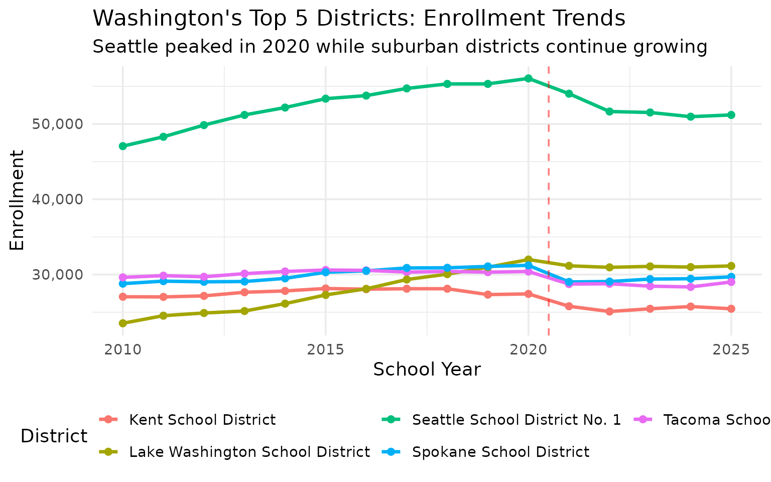
3. White students dropped from 64% to 48% as Hispanic enrollment nearly doubled
The state’s demographics reflect Pacific Rim immigration and a growing Hispanic population that rose from 167K to 295K students.
demographics <- enr |>
  filter(is_state, grade_level == "TOTAL",
         subgroup %in% c("white", "hispanic", "asian", "black", "multiracial"),
         end_year %in% c(2010, 2015, 2020, 2025)) |>
  select(end_year, subgroup, n_students, pct) |>
  mutate(pct = round(pct * 100, 1))
stopifnot(nrow(demographics) > 0)

demographics |>
  pivot_wider(names_from = end_year, values_from = c(n_students, pct))
#> # A tibble: 5 × 9
#>   subgroup    n_students_2010 n_students_2015 n_students_2020 n_students_2025
#>   <chr>                 <dbl>           <dbl>           <dbl>           <dbl>
#> 1 white                657143          615697          601749          526102
#> 2 black                 56515           48578           50251           53176
#> 3 hispanic             167426          235730          273842          294985
#> 4 asian                 80375           77981           91377          100676
#> 5 multiracial           35867           81757          101807          101068
#> # ℹ 4 more variables: pct_2010 <dbl>, pct_2015 <dbl>, pct_2020 <dbl>,
#> #   pct_2025 <dbl>
demo_trend <- enr |>
  filter(is_state, grade_level == "TOTAL",
         subgroup %in% c("white", "hispanic", "asian", "black", "multiracial"))
stopifnot(nrow(demo_trend) > 0)

print(demo_trend |> filter(end_year == 2025) |> select(subgroup, n_students, pct))
#>      subgroup n_students        pct
#> 1       white     526102 0.47594501
#> 2       black      53176 0.04810636
#> 3    hispanic     294985 0.26686201
#> 4       asian     100676 0.09107785
#> 5 multiracial     101068 0.09143248

ggplot(demo_trend, aes(x = end_year, y = pct * 100, color = subgroup)) +
  geom_line(linewidth = 1.2) +
  geom_point(size = 2) +
  scale_y_continuous(labels = function(x) paste0(x, "%")) +
  scale_color_brewer(palette = "Set2",
                     labels = c("Asian", "Black", "Hispanic", "Multiracial", "White")) +
  labs(
    title = "Washington's Shifting Demographics (2010-2025)",
    subtitle = "White enrollment declining as Hispanic and multiracial populations grow",
    x = "School Year",
    y = "Percent of Students",
    color = "Race/Ethnicity"
  ) +
  theme(legend.position = "bottom")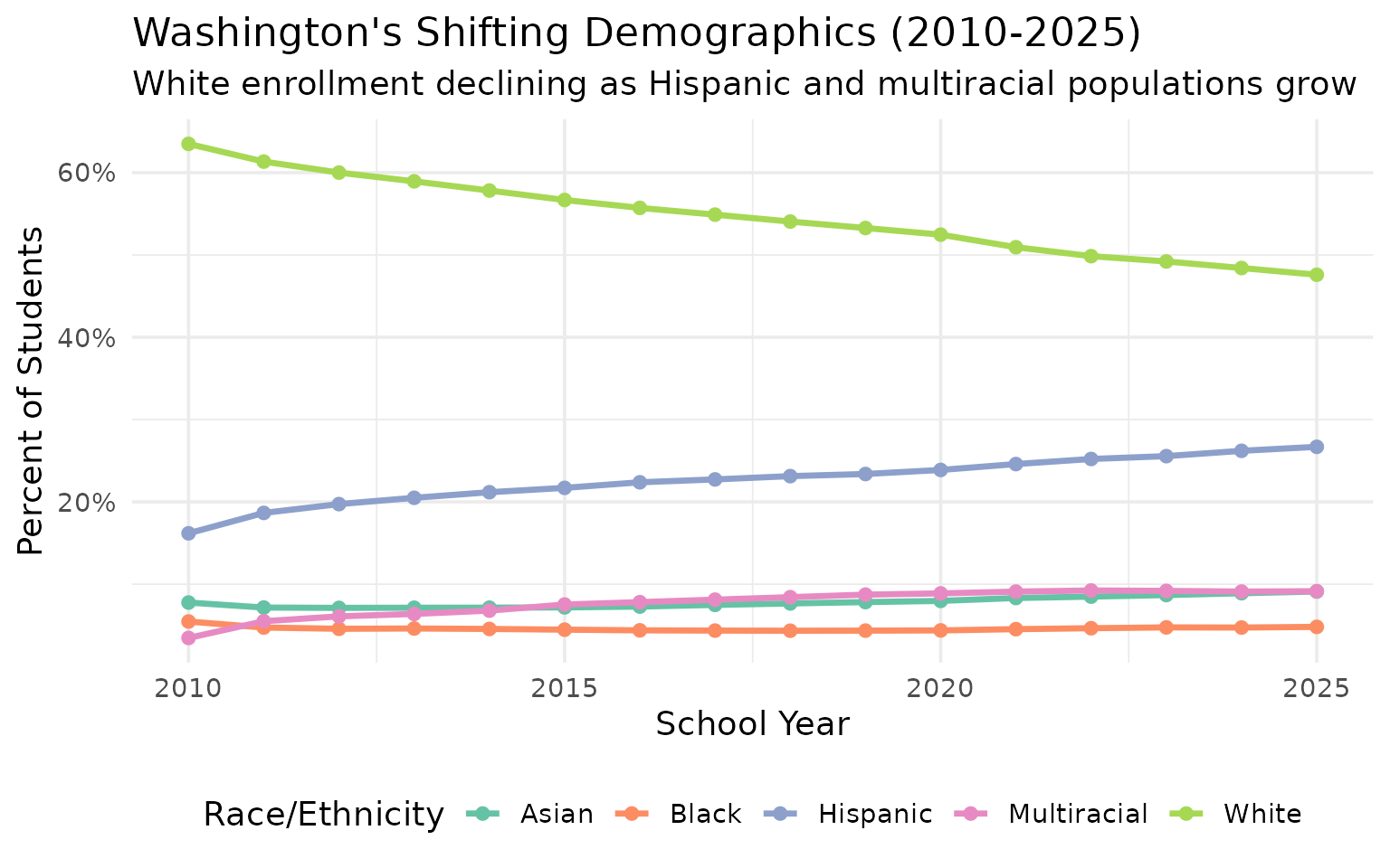
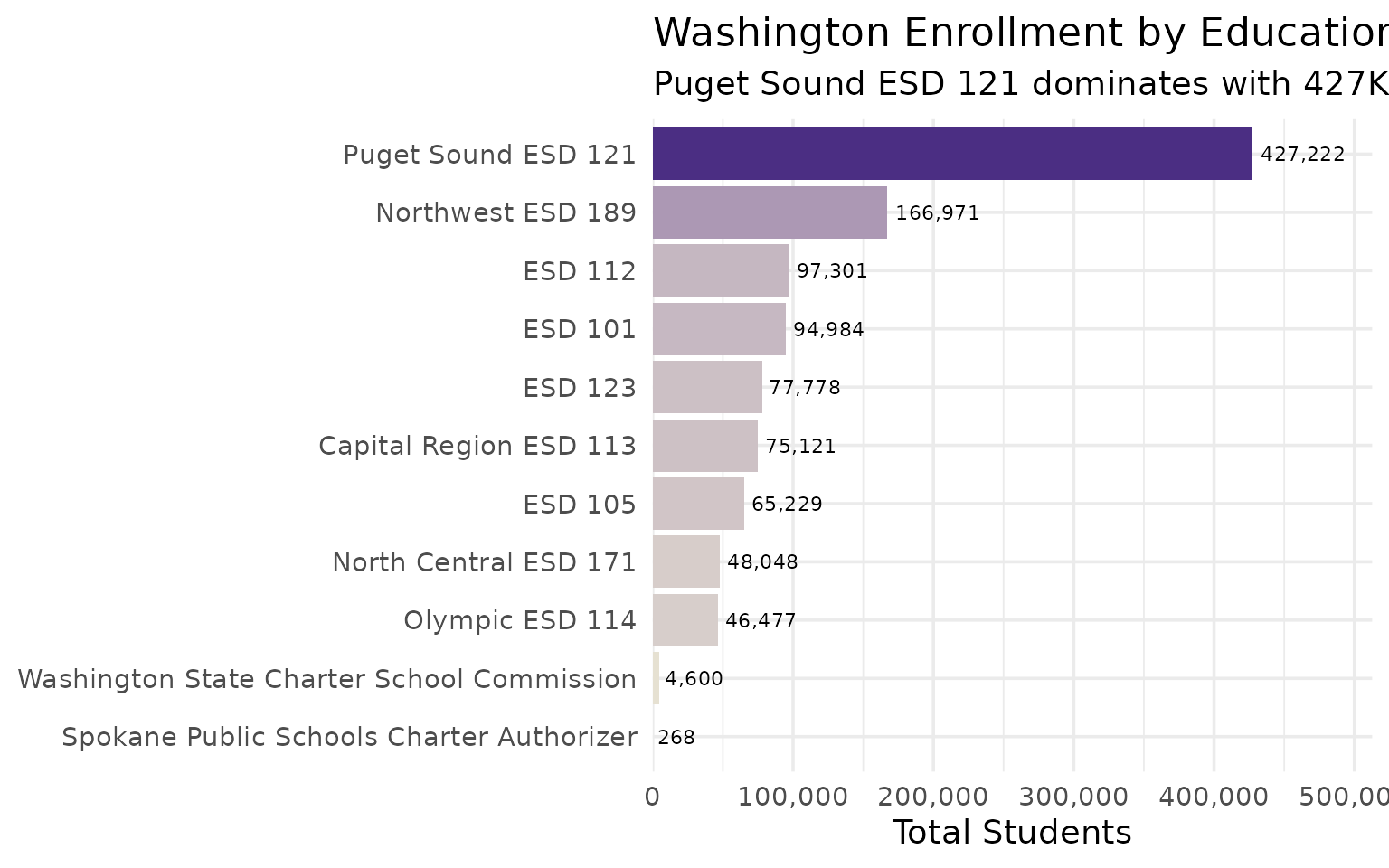
4. Puget Sound holds 427K students – nearly 4x Eastern Washington
The I-5 corridor dominates enrollment, but Eastern Washington’s districts face different challenges.
esd_enrollment <- enr |>
  filter(is_district, subgroup == "total_enrollment", grade_level == "TOTAL",
         end_year == 2025, !is.na(esd_name)) |>
  group_by(esd_name) |>
  summarize(
    districts = n(),
    students = sum(n_students, na.rm = TRUE),
    .groups = "drop"
  ) |>
  arrange(desc(students))
stopifnot(nrow(esd_enrollment) > 0)

esd_enrollment
#> # A tibble: 11 × 3
#>    esd_name                                       districts students
#>    <chr>                                              <int>    <dbl>
#>  1 Puget Sound Educational Service District 121          35   427222
#>  2 Northwest Educational Service District 189            35   166971
#>  3 Educational Service District 112                      30    97301
#>  4 Educational Service District 101                      59    94984
#>  5 Educational Service District 123                      22    77778
#>  6 Capital Region ESD 113                                44    75121
#>  7 Educational Service District 105                      25    65229
#>  8 North Central Educational Service District 171        29    48048
#>  9 Olympic Educational Service District 114              15    46477
#> 10 Washington State Charter School Commission            15     4600
#> 11 Spokane Public Schools Charter Authorizer              2      268
print(esd_enrollment)
#> # A tibble: 11 × 3
#>    esd_name                                       districts students
#>    <chr>                                              <int>    <dbl>
#>  1 Puget Sound Educational Service District 121          35   427222
#>  2 Northwest Educational Service District 189            35   166971
#>  3 Educational Service District 112                      30    97301
#>  4 Educational Service District 101                      59    94984
#>  5 Educational Service District 123                      22    77778
#>  6 Capital Region ESD 113                                44    75121
#>  7 Educational Service District 105                      25    65229
#>  8 North Central Educational Service District 171        29    48048
#>  9 Olympic Educational Service District 114              15    46477
#> 10 Washington State Charter School Commission            15     4600
#> 11 Spokane Public Schools Charter Authorizer              2      268

esd_enrollment |>
  mutate(esd_short = gsub("Educational Service District|ESD", "ESD", esd_name)) |>
  mutate(esd_short = forcats::fct_reorder(esd_short, students)) |>
  ggplot(aes(x = students, y = esd_short, fill = students)) +
  geom_col(show.legend = FALSE) +
  geom_text(aes(label = scales::comma(students)), hjust = -0.1, size = 3) +
  scale_x_continuous(labels = scales::comma, expand = expansion(mult = c(0, 0.2))) +
  scale_fill_gradient(low = "#E8E3D3", high = "#4B2E83") +
  labs(
    title = "Washington Enrollment by Educational Service District",
    subtitle = "Puget Sound ESD 121 dominates with 427K students",
    x = "Total Students",
    y = NULL
  )
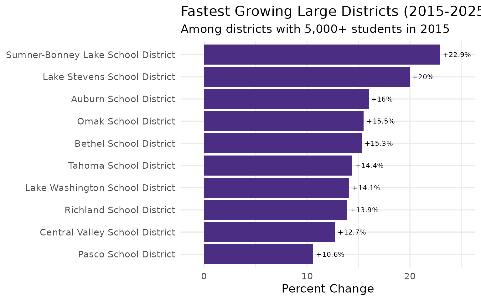
5. Suburban districts are booming: Sumner-Bonney Lake up 23% since 2015
The fastest-growing large districts are spread across the state, from Sumner-Bonney Lake south of Seattle to Central Valley near Spokane.
growth_rates <- enr |>
  filter(is_district, subgroup == "total_enrollment", grade_level == "TOTAL",
         end_year %in% c(2015, 2025)) |>
  select(district_id, district_name, end_year, n_students) |>
  pivot_wider(names_from = end_year, values_from = n_students, names_prefix = "yr_") |>
  filter(yr_2015 > 5000) |>
  mutate(
    change = yr_2025 - yr_2015,
    pct_change = round((yr_2025 - yr_2015) / yr_2015 * 100, 1)
  ) |>
  arrange(desc(pct_change))
stopifnot(nrow(growth_rates) > 0)

head(growth_rates, 10)
#> # A tibble: 10 × 6
#>    district_id district_name                   yr_2015 yr_2025 change pct_change
#>    <chr>       <chr>                             <dbl>   <dbl>  <dbl>      <dbl>
#>  1 100259      Sumner-Bonney Lake School Dist…    8988   11048   2060       22.9
#>  2 100126      Lake Stevens School District       8515   10215   1700       20
#>  3 100016      Auburn School District            15722   18234   2512       16
#>  4 100183      Omak School District               5257    6071    814       15.5
#>  5 100022      Bethel School District            18678   21538   2860       15.3
#>  6 100263      Tahoma School District             8118    9286   1168       14.4
#>  7 100127      Lake Washington School District   27293   31146   3853       14.1
#>  8 100218      Richland School District          12729   14499   1770       13.9
#>  9 100039      Central Valley School District    13396   15102   1706       12.7
#> 10 100195      Pasco School District             17182   19001   1819       10.6
growth_top10 <- head(growth_rates, 10)
print(growth_top10)
#> # A tibble: 10 × 6
#>    district_id district_name                   yr_2015 yr_2025 change pct_change
#>    <chr>       <chr>                             <dbl>   <dbl>  <dbl>      <dbl>
#>  1 100259      Sumner-Bonney Lake School Dist…    8988   11048   2060       22.9
#>  2 100126      Lake Stevens School District       8515   10215   1700       20
#>  3 100016      Auburn School District            15722   18234   2512       16
#>  4 100183      Omak School District               5257    6071    814       15.5
#>  5 100022      Bethel School District            18678   21538   2860       15.3
#>  6 100263      Tahoma School District             8118    9286   1168       14.4
#>  7 100127      Lake Washington School District   27293   31146   3853       14.1
#>  8 100218      Richland School District          12729   14499   1770       13.9
#>  9 100039      Central Valley School District    13396   15102   1706       12.7
#> 10 100195      Pasco School District             17182   19001   1819       10.6

growth_top10 |>
  mutate(district_name = forcats::fct_reorder(district_name, pct_change)) |>
  ggplot(aes(x = pct_change, y = district_name, fill = pct_change > 0)) +
  geom_col(show.legend = FALSE) +
  geom_text(aes(label = paste0("+", pct_change, "%")),
            hjust = -0.1, size = 3) +
  scale_x_continuous(expand = expansion(mult = c(0.1, 0.15))) +
  scale_fill_manual(values = c("TRUE" = "#4B2E83", "FALSE" = "#C4A055")) +
  labs(
    title = "Fastest Growing Large Districts (2015-2025)",
    subtitle = "Among districts with 5,000+ students in 2015",
    x = "Percent Change",
    y = NULL
  )
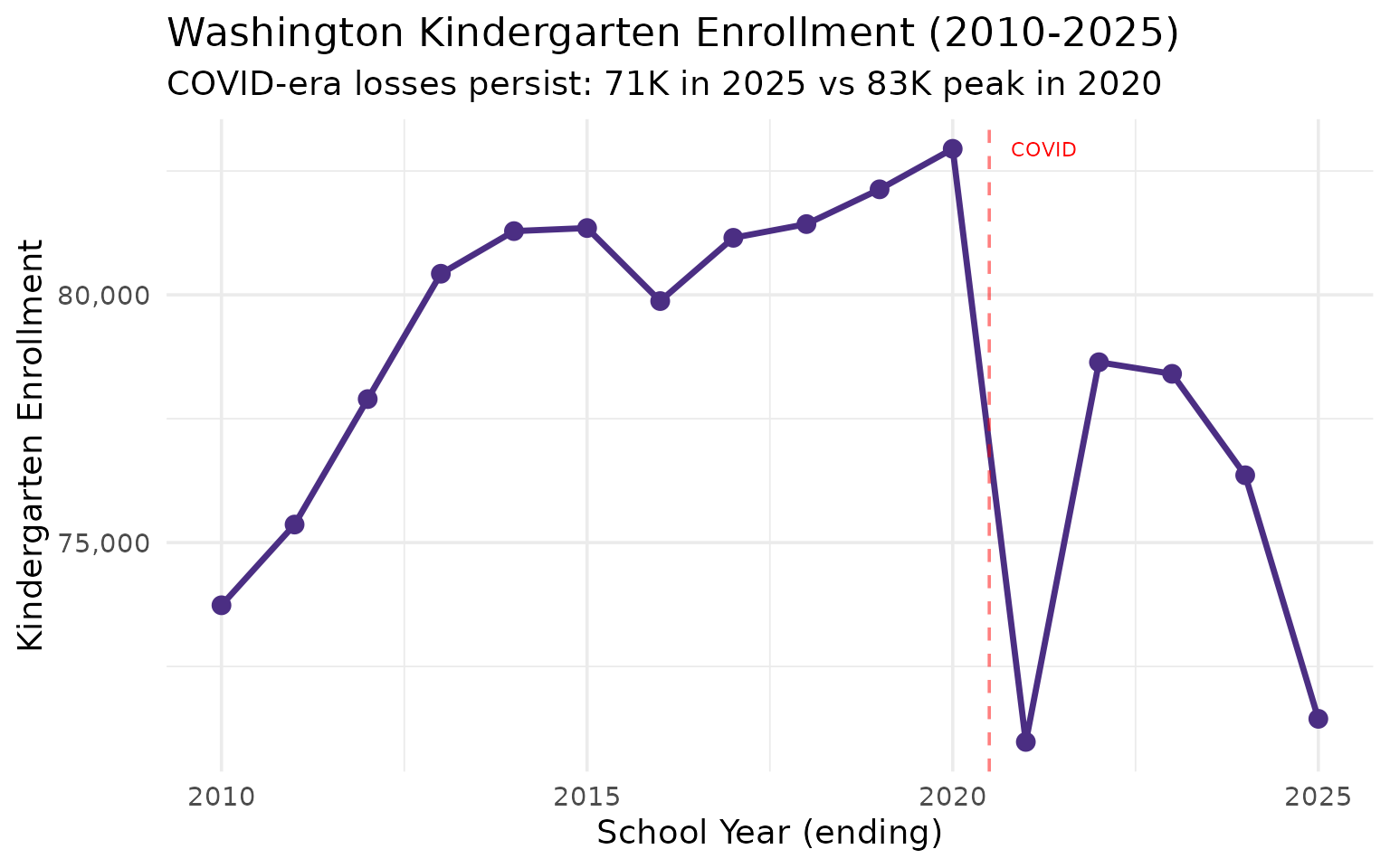
6. The kindergarten cliff is real: K enrollment down 14% from 2020 peak
Washington’s kindergarten enrollment dropped during COVID and hasn’t recovered, signaling smaller cohorts ahead.
k_trend <- enr |>
  filter(is_state, subgroup == "total_enrollment", grade_level == "K") |>
  select(end_year, n_students) |>
  mutate(pct_of_peak = round(n_students / max(n_students) * 100, 1))
stopifnot(nrow(k_trend) > 0)

k_trend
#>    end_year n_students pct_of_peak
#> 1      2010      73735        88.9
#> 2      2011      75364        90.9
#> 3      2012      77896        93.9
#> 4      2013      80426        97.0
#> 5      2014      81286        98.0
#> 6      2015      81348        98.1
#> 7      2016      79874        96.3
#> 8      2017      81151        97.8
#> 9      2018      81428        98.2
#> 10     2019      82130        99.0
#> 11     2020      82947       100.0
#> 12     2021      70977        85.6
#> 13     2022      78640        94.8
#> 14     2023      78406        94.5
#> 15     2024      76359        92.1
#> 16     2025      71443        86.1
print(k_trend)
#>    end_year n_students pct_of_peak
#> 1      2010      73735        88.9
#> 2      2011      75364        90.9
#> 3      2012      77896        93.9
#> 4      2013      80426        97.0
#> 5      2014      81286        98.0
#> 6      2015      81348        98.1
#> 7      2016      79874        96.3
#> 8      2017      81151        97.8
#> 9      2018      81428        98.2
#> 10     2019      82130        99.0
#> 11     2020      82947       100.0
#> 12     2021      70977        85.6
#> 13     2022      78640        94.8
#> 14     2023      78406        94.5
#> 15     2024      76359        92.1
#> 16     2025      71443        86.1

ggplot(k_trend, aes(x = end_year, y = n_students)) +
  geom_line(linewidth = 1.2, color = "#4B2E83") +
  geom_point(size = 3, color = "#4B2E83") +
  geom_vline(xintercept = 2020.5, linetype = "dashed", color = "red", alpha = 0.5) +
  annotate("text", x = 2020.8, y = max(k_trend$n_students, na.rm = TRUE),
           label = "COVID", hjust = 0, color = "red", size = 3) +
  scale_y_continuous(labels = scales::comma) +
  labs(
    title = "Washington Kindergarten Enrollment (2010-2025)",
    subtitle = "COVID-era losses persist: 71K in 2025 vs 83K peak in 2020",
    x = "School Year (ending)",
    y = "Kindergarten Enrollment"
  )
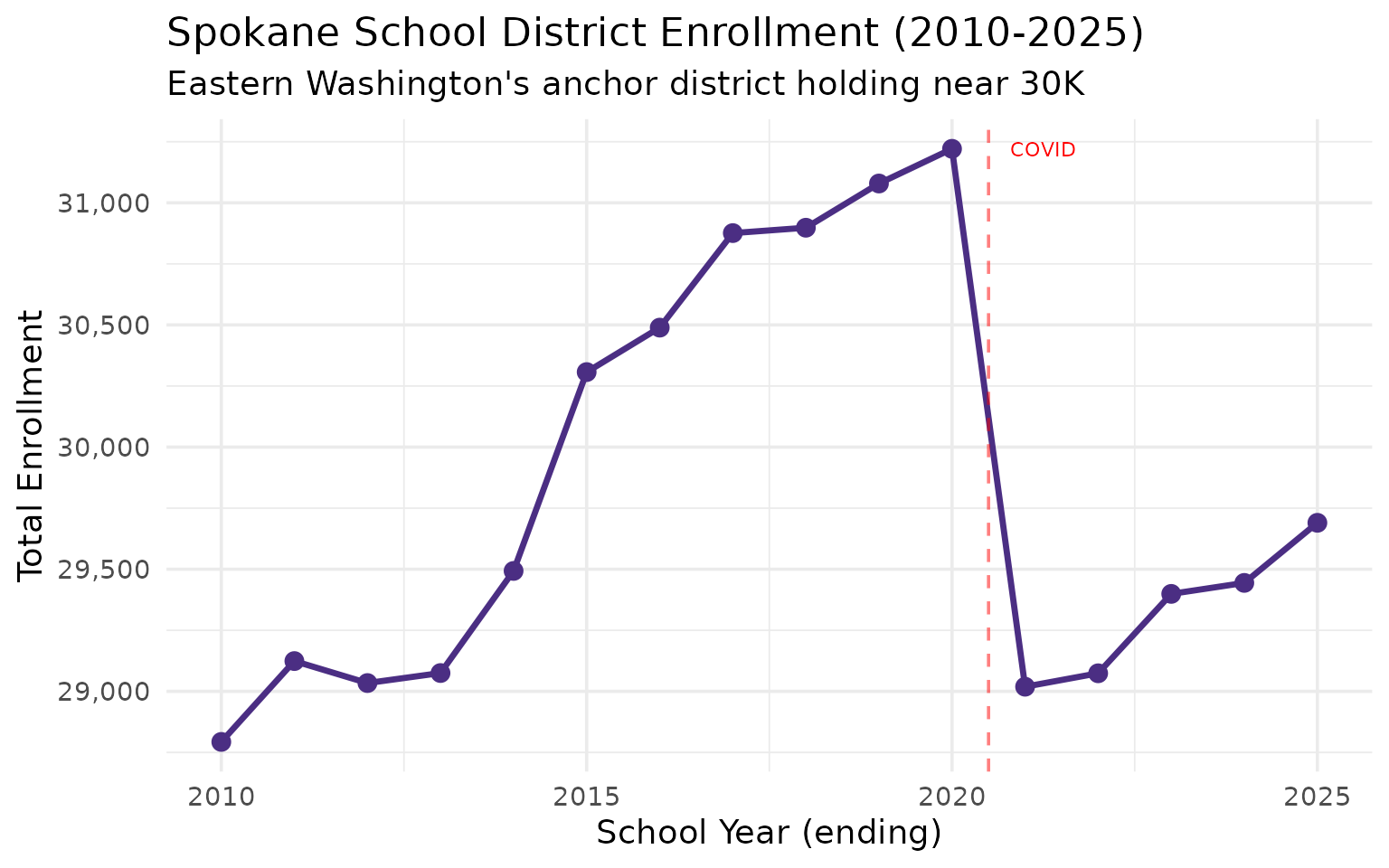
7. Spokane anchors Eastern Washington with nearly 30,000 students
Spokane Public Schools serves 29,690 students, making it the largest district east of the Cascades and the state’s second-largest overall.
spokane <- enr |>
  filter(is_district, subgroup == "total_enrollment", grade_level == "TOTAL",
         grepl("Spokane", district_name, ignore.case = TRUE),
         end_year == 2025) |>
  select(district_name, n_students) |>
  arrange(desc(n_students))
stopifnot(nrow(spokane) > 0)

spokane
#>                           district_name n_students
#> 1               Spokane School District      29690
#> 2 East Valley School District (Spokane)       3655
#> 3 West Valley School District (Spokane)       3501
#> 4         Spokane International Academy        830
#> 5            Innovation Spokane Schools        235
spokane_trend <- enr |>
  filter(is_district, subgroup == "total_enrollment", grade_level == "TOTAL",
         grepl("^Spokane School District$", district_name))
stopifnot(nrow(spokane_trend) > 0)

print(spokane_trend |> select(end_year, n_students))
#>    end_year n_students
#> 1      2010      28793
#> 2      2011      29124
#> 3      2012      29034
#> 4      2013      29075
#> 5      2014      29493
#> 6      2015      30307
#> 7      2016      30489
#> 8      2017      30876
#> 9      2018      30898
#> 10     2019      31079
#> 11     2020      31221
#> 12     2021      29019
#> 13     2022      29074
#> 14     2023      29399
#> 15     2024      29444
#> 16     2025      29690

ggplot(spokane_trend, aes(x = end_year, y = n_students)) +
  geom_line(linewidth = 1.2, color = "#4B2E83") +
  geom_point(size = 3, color = "#4B2E83") +
  geom_vline(xintercept = 2020.5, linetype = "dashed", color = "red", alpha = 0.5) +
  annotate("text", x = 2020.8, y = max(spokane_trend$n_students, na.rm = TRUE),
           label = "COVID", hjust = 0, color = "red", size = 3) +
  scale_y_continuous(labels = scales::comma) +
  labs(
    title = "Spokane School District Enrollment (2010-2025)",
    subtitle = "Eastern Washington's anchor district holding near 30K",
    x = "School Year (ending)",
    y = "Total Enrollment"
  )
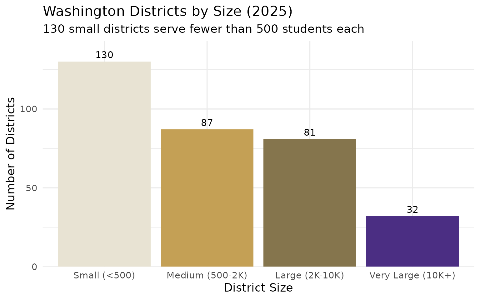
8. 130 districts have fewer than 500 students
Nearly 40% of Washington’s districts serve fewer than 500 students, challenging their long-term viability.
district_sizes <- enr |>
  filter(is_district, subgroup == "total_enrollment", grade_level == "TOTAL",
         end_year == 2025) |>
  mutate(size_bucket = case_when(
    n_students < 500 ~ "Small (<500)",
    n_students < 2000 ~ "Medium (500-2K)",
    n_students < 10000 ~ "Large (2K-10K)",
    TRUE ~ "Very Large (10K+)"
  )) |>
  count(size_bucket)
stopifnot(nrow(district_sizes) > 0)

district_sizes
#>         size_bucket   n
#> 1    Large (2K-10K)  81
#> 2   Medium (500-2K)  87
#> 3      Small (<500) 130
#> 4 Very Large (10K+)  32
print(district_sizes)
#>         size_bucket   n
#> 1    Large (2K-10K)  81
#> 2   Medium (500-2K)  87
#> 3      Small (<500) 130
#> 4 Very Large (10K+)  32

district_sizes |>
  mutate(size_bucket = factor(size_bucket,
    levels = c("Small (<500)", "Medium (500-2K)", "Large (2K-10K)", "Very Large (10K+)"))) |>
  ggplot(aes(x = size_bucket, y = n, fill = size_bucket)) +
  geom_col(show.legend = FALSE) +
  geom_text(aes(label = n), vjust = -0.5, size = 4) +
  scale_fill_manual(values = c("#E8E3D3", "#C4A055", "#85754D", "#4B2E83")) +
  scale_y_continuous(expand = expansion(mult = c(0, 0.1))) +
  labs(
    title = "Washington Districts by Size (2025)",
    subtitle = "130 small districts serve fewer than 500 students each",
    x = "District Size",
    y = "Number of Districts"
  )
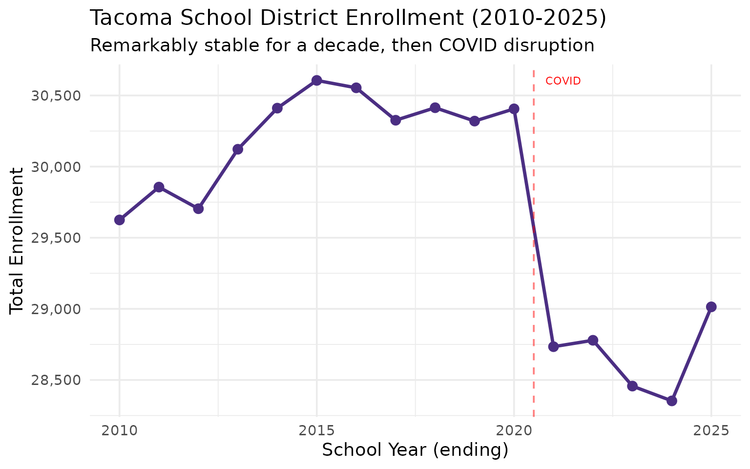
9. Tacoma held steady at ~30K for a decade before COVID
The state’s third-largest city maintained remarkably stable enrollment from 2010 to 2020 before losing 2,000 students.
tacoma <- enr |>
  filter(is_district, subgroup == "total_enrollment", grade_level == "TOTAL",
         grepl("Tacoma", district_name, ignore.case = TRUE)) |>
  select(end_year, district_name, n_students)
stopifnot(nrow(tacoma) > 0)

tacoma
#>    end_year          district_name n_students
#> 1      2010 Tacoma School District      29625
#> 2      2011 Tacoma School District      29856
#> 3      2012 Tacoma School District      29704
#> 4      2013 Tacoma School District      30122
#> 5      2014 Tacoma School District      30411
#> 6      2015 Tacoma School District      30606
#> 7      2016 Tacoma School District      30554
#> 8      2017 Tacoma School District      30326
#> 9      2018 Tacoma School District      30414
#> 10     2019 Tacoma School District      30320
#> 11     2020 Tacoma School District      30406
#> 12     2021 Tacoma School District      28734
#> 13     2022 Tacoma School District      28779
#> 14     2023 Tacoma School District      28457
#> 15     2024 Tacoma School District      28353
#> 16     2025 Tacoma School District      29014
print(tacoma)
#>    end_year          district_name n_students
#> 1      2010 Tacoma School District      29625
#> 2      2011 Tacoma School District      29856
#> 3      2012 Tacoma School District      29704
#> 4      2013 Tacoma School District      30122
#> 5      2014 Tacoma School District      30411
#> 6      2015 Tacoma School District      30606
#> 7      2016 Tacoma School District      30554
#> 8      2017 Tacoma School District      30326
#> 9      2018 Tacoma School District      30414
#> 10     2019 Tacoma School District      30320
#> 11     2020 Tacoma School District      30406
#> 12     2021 Tacoma School District      28734
#> 13     2022 Tacoma School District      28779
#> 14     2023 Tacoma School District      28457
#> 15     2024 Tacoma School District      28353
#> 16     2025 Tacoma School District      29014

ggplot(tacoma, aes(x = end_year, y = n_students)) +
  geom_line(linewidth = 1.2, color = "#4B2E83") +
  geom_point(size = 3, color = "#4B2E83") +
  geom_vline(xintercept = 2020.5, linetype = "dashed", color = "red", alpha = 0.5) +
  annotate("text", x = 2020.8, y = max(tacoma$n_students, na.rm = TRUE),
           label = "COVID", hjust = 0, color = "red", size = 3) +
  scale_y_continuous(labels = scales::comma) +
  labs(
    title = "Tacoma School District Enrollment (2010-2025)",
    subtitle = "Remarkably stable for a decade, then COVID disruption",
    x = "School Year (ending)",
    y = "Total Enrollment"
  )
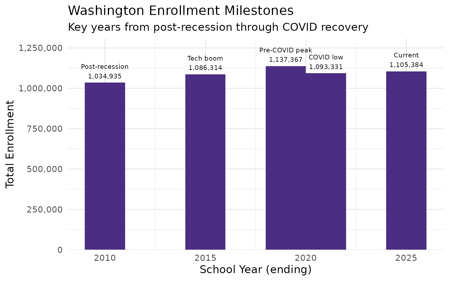
10. From 1.03M to 1.1M: 16 years of enrollment milestones
Washington’s enrollment data spans 2010-2025, documenting the tech boom, pandemic disruption, and demographic transformation.
decade_summary <- enr |>
  filter(is_state, subgroup == "total_enrollment", grade_level == "TOTAL",
         end_year %in% c(2010, 2015, 2019, 2021, 2025)) |>
  select(end_year, n_students) |>
  mutate(label = case_when(
    end_year == 2010 ~ "Post-recession",
    end_year == 2015 ~ "Tech boom",
    end_year == 2019 ~ "Pre-COVID peak",
    end_year == 2021 ~ "COVID low",
    end_year == 2025 ~ "Current"
  ))
stopifnot(nrow(decade_summary) > 0)

decade_summary
#>   end_year n_students          label
#> 1     2010    1034935 Post-recession
#> 2     2015    1086314      Tech boom
#> 3     2019    1137367 Pre-COVID peak
#> 4     2021    1093331      COVID low
#> 5     2025    1105384        Current
print(decade_summary)
#>   end_year n_students          label
#> 1     2010    1034935 Post-recession
#> 2     2015    1086314      Tech boom
#> 3     2019    1137367 Pre-COVID peak
#> 4     2021    1093331      COVID low
#> 5     2025    1105384        Current

ggplot(decade_summary, aes(x = end_year, y = n_students)) +
  geom_col(fill = "#4B2E83", width = 2) +
  geom_text(aes(label = paste0(label, "\n", scales::comma(n_students))),
            vjust = -0.3, size = 3) +
  scale_y_continuous(labels = scales::comma, expand = expansion(mult = c(0, 0.15))) +
  labs(
    title = "Washington Enrollment Milestones",
    subtitle = "Key years from post-recession through COVID recovery",
    x = "School Year (ending)",
    y = "Total Enrollment"
  )
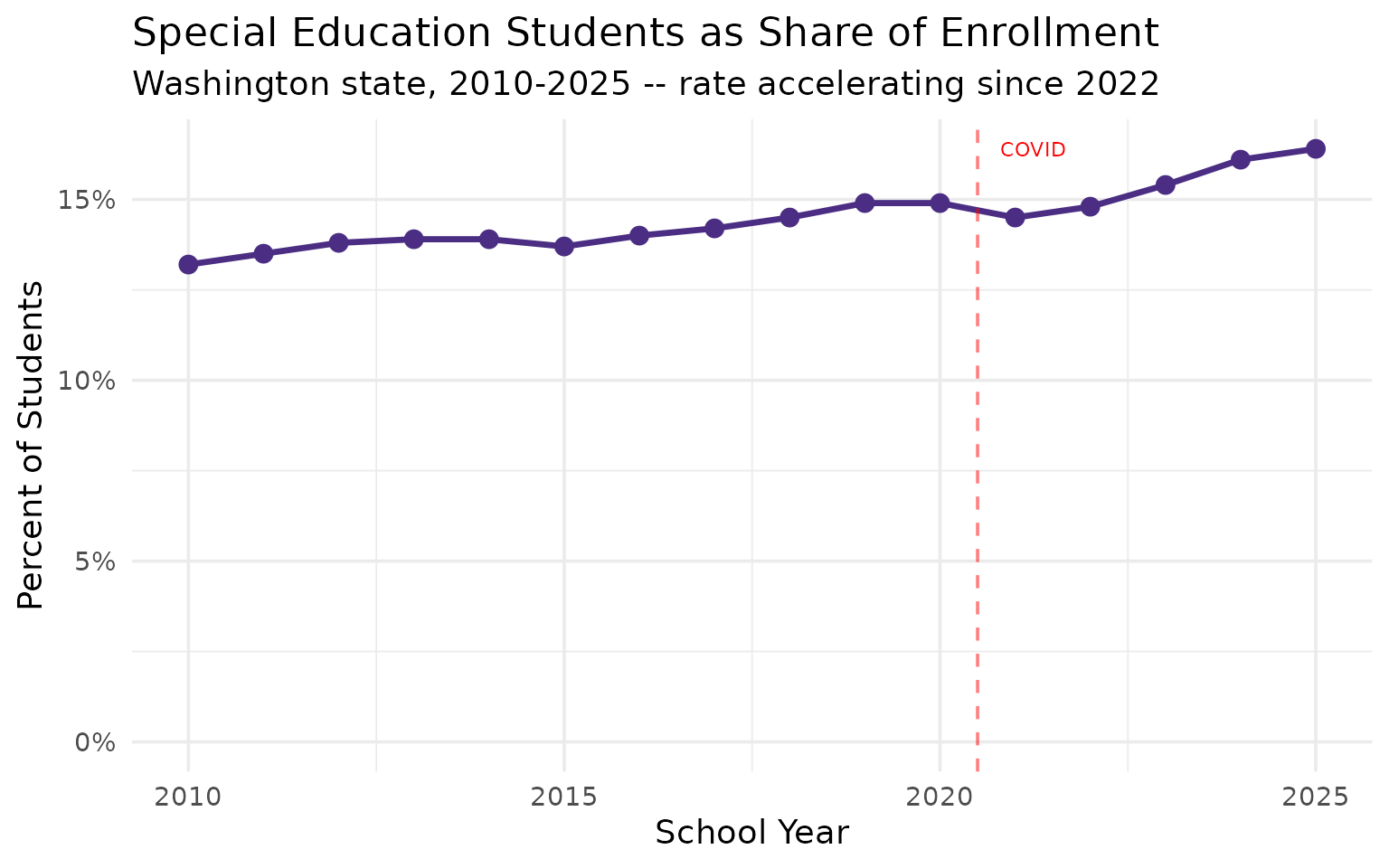
11. 1 in 6 Washington students now receives special education services
Special education identification rose from 13.2% to 16.4% over 16 years, with the rate accelerating since 2022.
sped_trend <- enr |>
  filter(is_state, grade_level == "TOTAL", subgroup == "special_ed") |>
  select(end_year, n_students, pct) |>
  mutate(pct = round(pct * 100, 1))
stopifnot(nrow(sped_trend) > 0)

sped_trend
#>    end_year n_students  pct
#> 1      2010     136129 13.2
#> 2      2011     141583 13.5
#> 3      2012     145177 13.8
#> 4      2013     146773 13.9
#> 5      2014     148462 13.9
#> 6      2015     149314 13.7
#> 7      2016     153648 14.0
#> 8      2017     157984 14.2
#> 9      2018     163839 14.5
#> 10     2019     169270 14.9
#> 11     2020     170961 14.9
#> 12     2021     158218 14.5
#> 13     2022     161967 14.8
#> 14     2023     168599 15.4
#> 15     2024     176801 16.1
#> 16     2025     181381 16.4
print(sped_trend)
#>    end_year n_students  pct
#> 1      2010     136129 13.2
#> 2      2011     141583 13.5
#> 3      2012     145177 13.8
#> 4      2013     146773 13.9
#> 5      2014     148462 13.9
#> 6      2015     149314 13.7
#> 7      2016     153648 14.0
#> 8      2017     157984 14.2
#> 9      2018     163839 14.5
#> 10     2019     169270 14.9
#> 11     2020     170961 14.9
#> 12     2021     158218 14.5
#> 13     2022     161967 14.8
#> 14     2023     168599 15.4
#> 15     2024     176801 16.1
#> 16     2025     181381 16.4

ggplot(sped_trend, aes(x = end_year, y = pct)) +
  geom_line(linewidth = 1.2, color = "#4B2E83") +
  geom_point(size = 3, color = "#4B2E83") +
  geom_vline(xintercept = 2020.5, linetype = "dashed", color = "red", alpha = 0.5) +
  annotate("text", x = 2020.8, y = max(sped_trend$pct, na.rm = TRUE),
           label = "COVID", hjust = 0, color = "red", size = 3) +
  scale_y_continuous(labels = function(x) paste0(x, "%"),
                     limits = c(0, NA)) +
  labs(
    title = "Special Education Students as Share of Enrollment",
    subtitle = "Washington state, 2010-2025 -- rate accelerating since 2022",
    x = "School Year",
    y = "Percent of Students"
  )
12. Yakima Valley: where 93% of students are Hispanic and half are English learners
Central Washington’s agricultural heartland has the state’s highest concentrations of English learners and economically disadvantaged students.
yakima_districts <- enr |>
  filter(is_district, grade_level == "TOTAL", end_year == 2025,
         grepl("Yakima|Sunnyside|Toppenish|Wapato|Grandview", district_name)) |>
  select(district_name, subgroup, n_students) |>
  pivot_wider(names_from = subgroup, values_from = n_students) |>
  mutate(
    pct_hispanic = round(hispanic / total_enrollment * 100, 1),
    pct_ell = round(lep / total_enrollment * 100, 1),
    pct_econ_disadv = round(econ_disadv / total_enrollment * 100, 1)
  ) |>
  select(district_name, total_enrollment, pct_hispanic, pct_ell, pct_econ_disadv) |>
  arrange(desc(total_enrollment))
stopifnot(nrow(yakima_districts) > 0)

yakima_districts
#> # A tibble: 7 × 5
#>   district_name            total_enrollment pct_hispanic pct_ell pct_econ_disadv
#>   <chr>                               <dbl>        <dbl>   <dbl>           <dbl>
#> 1 Yakima School District              15621         82.1    34.2            86.8
#> 2 Sunnyside School Distri…             6169         92.9    33.3            87.6
#> 3 West Valley School Dist…             5570         41.5     9.9            54.9
#> 4 Toppenish School Distri…             3670         86.9    36.3            89.9
#> 5 Grandview School Distri…             3586         93.4    32.7            85.5
#> 6 East Valley School Dist…             3408         58.5    15              65.7
#> 7 Wapato School District               3225         77.2    50.6            89.9
yakima_long <- enr |>
  filter(is_district, grade_level == "TOTAL", end_year == 2025,
         grepl("Yakima|Sunnyside|Toppenish|Wapato|Grandview", district_name),
         subgroup %in% c("hispanic", "lep", "econ_disadv")) |>
  select(district_name, subgroup, pct) |>
  mutate(pct = pct * 100,
         subgroup = case_when(
           subgroup == "hispanic" ~ "Hispanic",
           subgroup == "lep" ~ "English Learner",
           subgroup == "econ_disadv" ~ "Economically Disadvantaged"
         ))
stopifnot(nrow(yakima_long) > 0)

print(yakima_long)
#>                           district_name                   subgroup      pct
#> 1                Yakima School District                   Hispanic 82.14583
#> 2  East Valley School District (Yakima)                   Hispanic 58.45070
#> 3             Grandview School District                   Hispanic 93.41885
#> 4             Sunnyside School District                   Hispanic 92.89998
#> 5             Toppenish School District                   Hispanic 86.86649
#> 6                Wapato School District                   Hispanic 77.17829
#> 7  West Valley School District (Yakima)                   Hispanic 41.50808
#> 8                Yakima School District            English Learner 34.19115
#> 9  East Valley School District (Yakima)            English Learner 14.99413
#> 10            Grandview School District            English Learner 32.71054
#> 11            Sunnyside School District            English Learner 33.34414
#> 12            Toppenish School District            English Learner 36.32153
#> 13               Wapato School District            English Learner 50.57364
#> 14 West Valley School District (Yakima)            English Learner  9.94614
#> 15               Yakima School District Economically Disadvantaged 86.83183
#> 16 East Valley School District (Yakima) Economically Disadvantaged 65.66901
#> 17            Grandview School District Economically Disadvantaged 85.52705
#> 18            Sunnyside School District Economically Disadvantaged 87.59929
#> 19            Toppenish School District Economically Disadvantaged 89.89101
#> 20               Wapato School District Economically Disadvantaged 89.86047
#> 21 West Valley School District (Yakima) Economically Disadvantaged 54.93716

ggplot(yakima_long, aes(x = reorder(district_name, -pct), y = pct, fill = subgroup)) +
  geom_col(position = "dodge") +
  scale_fill_brewer(palette = "Set2") +
  labs(
    title = "Yakima Valley Districts: Demographics",
    subtitle = "High concentrations of Hispanic, ELL, and low-income students",
    x = NULL,
    y = "Percent of Students",
    fill = "Subgroup"
  ) +
  theme(axis.text.x = element_text(angle = 45, hjust = 1),
        legend.position = "bottom")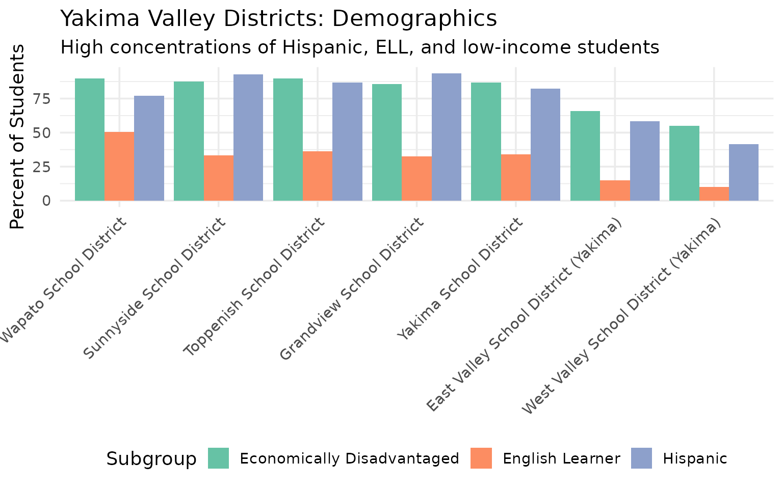
13. Ridgefield grew 84% while Vancouver lost 7% – Clark County’s diverging paths
The Portland metro spillover has reshaped Clark County, with small suburban districts booming while the urban core declines.
clark_districts <- enr |>
  filter(is_district, subgroup == "total_enrollment", grade_level == "TOTAL",
         grepl("Vancouver|Evergreen SD|Camas|Battle Ground|Ridgefield", district_name),
         end_year %in% c(2015, 2020, 2025)) |>
  select(district_name, end_year, n_students) |>
  pivot_wider(names_from = end_year, values_from = n_students, names_prefix = "yr_") |>
  mutate(
    growth_2015_2025 = round((yr_2025 - yr_2015) / yr_2015 * 100, 1)
  ) |>
  arrange(desc(growth_2015_2025))
stopifnot(nrow(clark_districts) > 0)

clark_districts
#> # A tibble: 4 × 5
#>   district_name                 yr_2015 yr_2020 yr_2025 growth_2015_2025
#>   <chr>                           <dbl>   <dbl>   <dbl>            <dbl>
#> 1 Ridgefield School District       2343    3499    4315             84.2
#> 2 Camas School District            6695    7654    7272              8.6
#> 3 Battle Ground School District   13589   13365   13080             -3.7
#> 4 Vancouver School District       23486   23404   21943             -6.6
clark_trend <- enr |>
  filter(is_district, subgroup == "total_enrollment", grade_level == "TOTAL",
         grepl("Vancouver|Evergreen SD|Camas|Battle Ground|Ridgefield", district_name))
stopifnot(nrow(clark_trend) > 0)

print(clark_trend |> filter(end_year == 2025) |> select(district_name, n_students))
#>                   district_name n_students
#> 1     Vancouver School District      21943
#> 2         Camas School District       7272
#> 3 Battle Ground School District      13080
#> 4    Ridgefield School District       4315

ggplot(clark_trend, aes(x = end_year, y = n_students, color = district_name)) +
  geom_line(linewidth = 1.2) +
  geom_point(size = 2) +
  geom_vline(xintercept = 2020.5, linetype = "dashed", color = "red", alpha = 0.5) +
  scale_y_continuous(labels = scales::comma) +
  scale_color_brewer(palette = "Set1") +
  labs(
    title = "Clark County District Enrollment Trends",
    subtitle = "Ridgefield booming while Vancouver declines",
    x = "School Year",
    y = "Enrollment",
    color = "District"
  ) +
  theme(legend.position = "bottom") +
  guides(color = guide_legend(nrow = 2))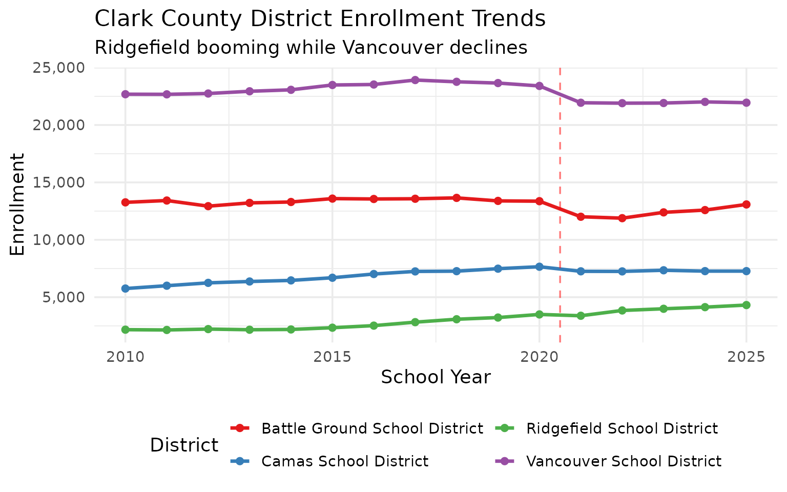
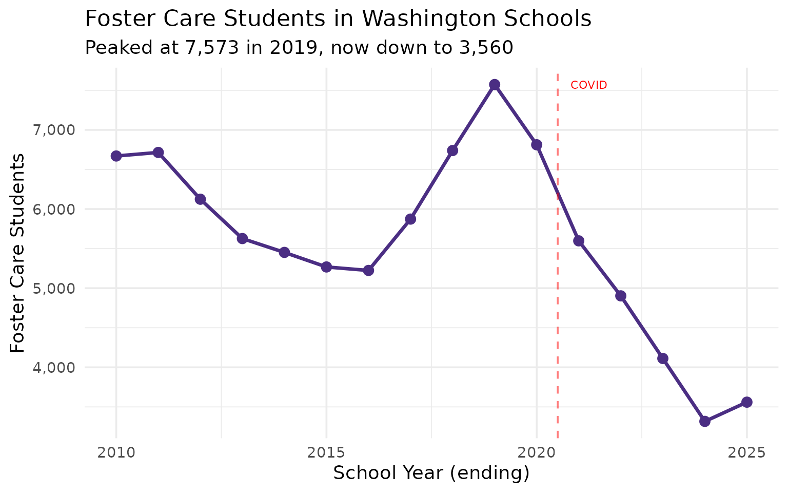
14. Foster care enrollment dropped 53% from 2019 peak
Washington tracks foster care enrollment at every school, revealing the population peaked at 7,573 in 2019 and has since dropped to 3,560.
foster_trend <- enr |>
  filter(is_state, grade_level == "TOTAL", subgroup == "foster_care") |>
  select(end_year, n_students, pct) |>
  mutate(pct = round(pct * 100, 2))
stopifnot(nrow(foster_trend) > 0)

foster_trend
#>    end_year n_students  pct
#> 1      2010       6670 0.64
#> 2      2011       6715 0.64
#> 3      2012       6124 0.58
#> 4      2013       5627 0.53
#> 5      2014       5452 0.51
#> 6      2015       5268 0.48
#> 7      2016       5224 0.47
#> 8      2017       5873 0.53
#> 9      2018       6739 0.60
#> 10     2019       7573 0.67
#> 11     2020       6812 0.59
#> 12     2021       5598 0.51
#> 13     2022       4903 0.45
#> 14     2023       4112 0.37
#> 15     2024       3317 0.30
#> 16     2025       3560 0.32
print(foster_trend)
#>    end_year n_students  pct
#> 1      2010       6670 0.64
#> 2      2011       6715 0.64
#> 3      2012       6124 0.58
#> 4      2013       5627 0.53
#> 5      2014       5452 0.51
#> 6      2015       5268 0.48
#> 7      2016       5224 0.47
#> 8      2017       5873 0.53
#> 9      2018       6739 0.60
#> 10     2019       7573 0.67
#> 11     2020       6812 0.59
#> 12     2021       5598 0.51
#> 13     2022       4903 0.45
#> 14     2023       4112 0.37
#> 15     2024       3317 0.30
#> 16     2025       3560 0.32

ggplot(foster_trend, aes(x = end_year, y = n_students)) +
  geom_line(linewidth = 1.2, color = "#4B2E83") +
  geom_point(size = 3, color = "#4B2E83") +
  geom_vline(xintercept = 2020.5, linetype = "dashed", color = "red", alpha = 0.5) +
  annotate("text", x = 2020.8, y = max(foster_trend$n_students, na.rm = TRUE),
           label = "COVID", hjust = 0, color = "red", size = 3) +
  scale_y_continuous(labels = scales::comma) +
  labs(
    title = "Foster Care Students in Washington Schools",
    subtitle = "Peaked at 7,573 in 2019, now down to 3,560",
    x = "School Year (ending)",
    y = "Foster Care Students"
  )
15. The Tri-Cities boom: Pasco grew 31% while Kennewick and Richland added 19% and 32%
The Tri-Cities in southeastern Washington have seen sustained population growth driven by Hanford cleanup and agricultural expansion.
tri_cities <- enr |>
  filter(is_district, subgroup == "total_enrollment", grade_level == "TOTAL",
         grepl("Richland|Kennewick|Pasco", district_name)) |>
  select(end_year, district_name, n_students)
stopifnot(nrow(tri_cities) > 0)

tri_cities_wide <- tri_cities |>
  filter(end_year %in% c(2010, 2015, 2020, 2025)) |>
  pivot_wider(names_from = end_year, values_from = n_students, names_prefix = "yr_")

tri_cities_wide
#> # A tibble: 3 × 5
#>   district_name             yr_2010 yr_2015 yr_2020 yr_2025
#>   <chr>                       <dbl>   <dbl>   <dbl>   <dbl>
#> 1 Kennewick School District   16085   17611   19554   19109
#> 2 Pasco School District       14473   17182   19226   19001
#> 3 Richland School District    10965   12729   14295   14499
print(tri_cities_wide)
#> # A tibble: 3 × 5
#>   district_name             yr_2010 yr_2015 yr_2020 yr_2025
#>   <chr>                       <dbl>   <dbl>   <dbl>   <dbl>
#> 1 Kennewick School District   16085   17611   19554   19109
#> 2 Pasco School District       14473   17182   19226   19001
#> 3 Richland School District    10965   12729   14295   14499

ggplot(tri_cities, aes(x = end_year, y = n_students, color = district_name)) +
  geom_line(linewidth = 1.2) +
  geom_point(size = 2) +
  geom_vline(xintercept = 2020.5, linetype = "dashed", color = "red", alpha = 0.5) +
  scale_y_continuous(labels = scales::comma) +
  scale_color_manual(values = c("Kennewick School District" = "#4B2E83",
                                "Pasco School District" = "#C4A055",
                                "Richland School District" = "#85754D"),
                     labels = function(x) gsub(" School District", "", x)) +
  labs(
    title = "Tri-Cities Enrollment Growth",
    subtitle = "Southeastern Washington's sustained growth region",
    x = "School Year",
    y = "Enrollment",
    color = "District"
  ) +
  theme(legend.position = "bottom")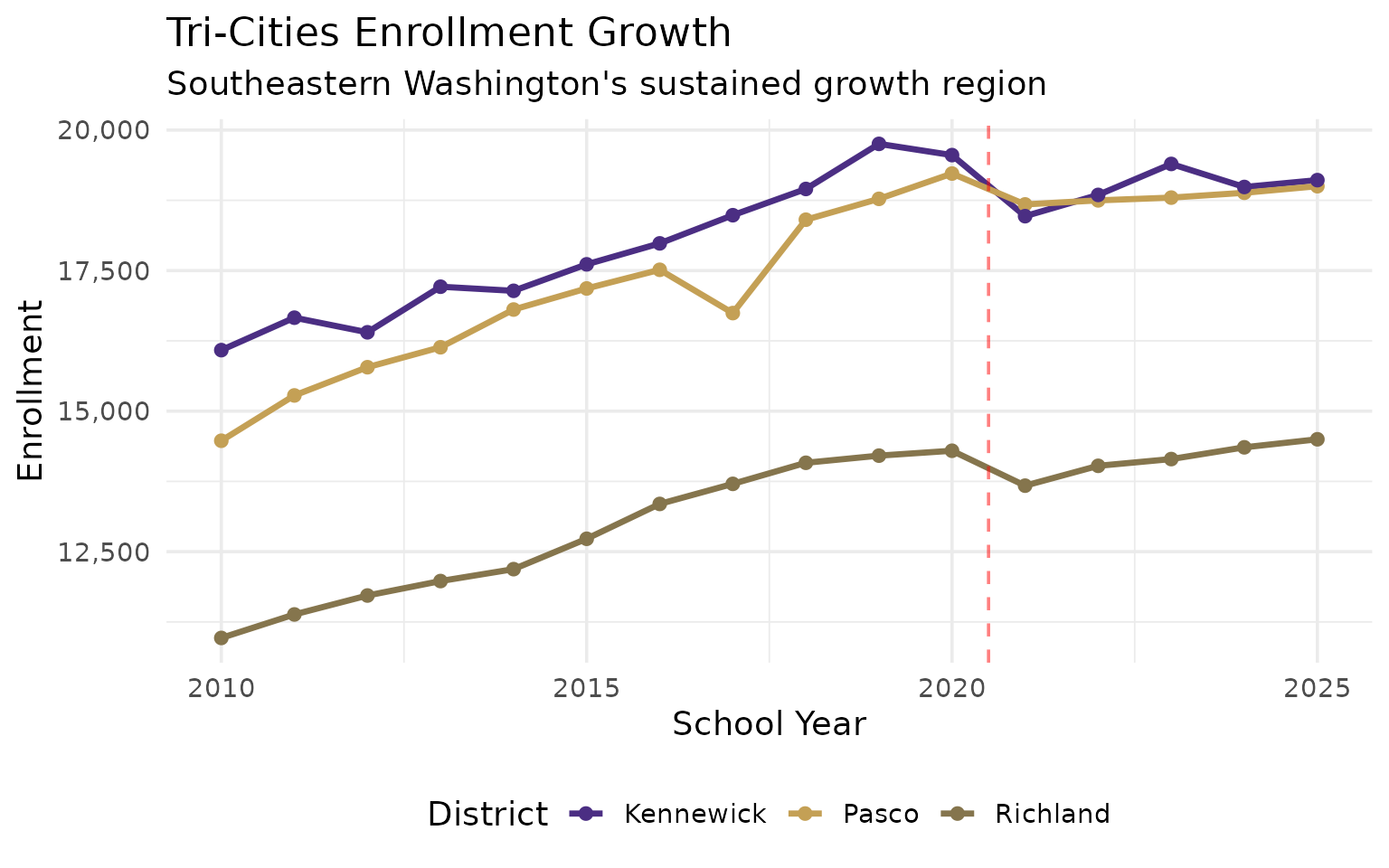
Summary
Washington’s school enrollment data reveals:
- Steady growth: 1.03M to 1.15M students over a decade before COVID
- Seattle paradox: The largest district lost 9% while suburban districts boomed
- Demographic transformation: White students dropped from 64% to 48%, Hispanic nearly doubled
- Kindergarten cliff: K enrollment down 14% from peak, signaling smaller future cohorts
- Rural pressure: 130 districts serve fewer than 500 students each
- Special education growth: Rising from 13% to 16% of all students
- Agricultural communities: Yakima Valley districts are 80-93% Hispanic
- Clark County divergence: Ridgefield up 84%, Vancouver down 7%
- Foster care decline: Peaked at 7,573 in 2019, now down 53%
- Tri-Cities expansion: All three districts grew 19-32% since 2010
These patterns shape school funding, facility planning, and staffing decisions across the Evergreen State.
Data sourced from the Washington Office of Superintendent of Public Instruction (OSPI) via the Washington State Report Card and data.wa.gov.
Session Info
sessionInfo()
#> R version 4.5.2 (2025-10-31)
#> Platform: x86_64-pc-linux-gnu
#> Running under: Ubuntu 24.04.3 LTS
#>
#> Matrix products: default
#> BLAS:   /usr/lib/x86_64-linux-gnu/openblas-pthread/libblas.so.3
#> LAPACK: /usr/lib/x86_64-linux-gnu/openblas-pthread/libopenblasp-r0.3.26.so;  LAPACK version 3.12.0
#>
#> locale:
#>  [1] LC_CTYPE=C.UTF-8       LC_NUMERIC=C           LC_TIME=C.UTF-8
#>  [4] LC_COLLATE=C.UTF-8     LC_MONETARY=C.UTF-8    LC_MESSAGES=C.UTF-8
#>  [7] LC_PAPER=C.UTF-8       LC_NAME=C              LC_ADDRESS=C
#> [10] LC_TELEPHONE=C         LC_MEASUREMENT=C.UTF-8 LC_IDENTIFICATION=C
#>
#> time zone: UTC
#> tzcode source: system (glibc)
#>
#> attached base packages:
#> [1] stats     graphics  grDevices utils     datasets  methods   base
#>
#> other attached packages:
#> [1] ggplot2_4.0.2      tidyr_1.3.2        dplyr_1.2.0        waschooldata_0.1.0
#> [5] testthat_3.3.2
#>
#> loaded via a namespace (and not attached):
#>  [1] gtable_0.3.6       jsonlite_2.0.0     compiler_4.5.2     brio_1.1.5
#>  [5] tidyselect_1.2.1   jquerylib_0.1.4    systemfonts_1.3.2  scales_1.4.0
#>  [9] textshaping_1.0.5  yaml_2.3.12        fastmap_1.2.0      R6_2.6.1
#> [13] labeling_0.4.3     generics_0.1.4     curl_7.0.0         knitr_1.51
#> [17] forcats_1.0.1      tibble_3.3.1       desc_1.4.3         bslib_0.10.0
#> [21] pillar_1.11.1      RColorBrewer_1.1-3 rlang_1.1.7        utf8_1.2.6
#> [25] cachem_1.1.0       xfun_0.56          S7_0.2.1           fs_1.6.7
#> [29] sass_0.4.10        cli_3.6.5          withr_3.0.2        pkgdown_2.2.0
#> [33] magrittr_2.0.4     digest_0.6.39      grid_4.5.2         rappdirs_0.3.4
#> [37] lifecycle_1.0.5    vctrs_0.7.1        evaluate_1.0.5     glue_1.8.0
#> [41] farver_2.1.2       codetools_0.2-20   ragg_1.5.1         httr_1.4.8
#> [45] rmarkdown_2.30     purrr_1.2.1        tools_4.5.2        pkgconfig_2.0.3
#> [49] htmltools_0.5.9