15 Insights from Wisconsin School Enrollment Data
Source:vignettes/enrollment_hooks.Rmd
enrollment_hooks.Rmd
library(wischooldata)
library(dplyr)
library(tidyr)
library(ggplot2)

theme_set(theme_minimal(base_size = 14))
This vignette explores Wisconsin’s public school enrollment data, surfacing key trends and demographic patterns across the Badger State’s school system.
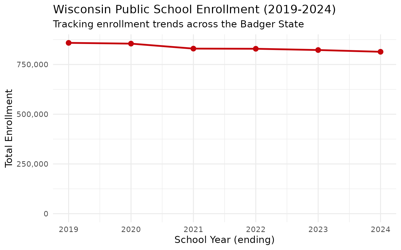
1. Wisconsin lost nearly 45,000 students since 2019
Wisconsin enrollment has declined every year since 2019, accelerating after the COVID-19 pandemic. The state has not recovered.
# NOTE: 2017-18 file excluded because WI DPI server returns HTTP 503 for that year
enr <- fetch_enr_multi(2019:2024, use_cache = TRUE)

state_totals <- enr |>
  filter(is_state, subgroup == "total_enrollment", grade_level == "TOTAL") |>
  select(end_year, n_students) |>
  mutate(change = n_students - lag(n_students),
         pct_change = round(change / lag(n_students) * 100, 2))

state_totals
#>   end_year n_students change pct_change
#> 1     2019     858833     NA         NA
#> 2     2020     854959  -3874      -0.45
#> 3     2021     829935 -25024      -2.93
#> 4     2022     829143   -792      -0.10
#> 5     2023     822804  -6339      -0.76
#> 6     2024     814002  -8802      -1.07
stopifnot(nrow(state_totals) > 0)
ggplot(state_totals, aes(x = end_year, y = n_students)) +
  geom_line(linewidth = 1.2, color = "#C5050C") +
  geom_point(size = 3, color = "#C5050C") +
  scale_y_continuous(labels = scales::comma, limits = c(0, NA)) +
  labs(
    title = "Wisconsin Public School Enrollment (2019-2024)",
    subtitle = "Tracking enrollment trends across the Badger State",
    x = "School Year (ending)",
    y = "Total Enrollment"
  )
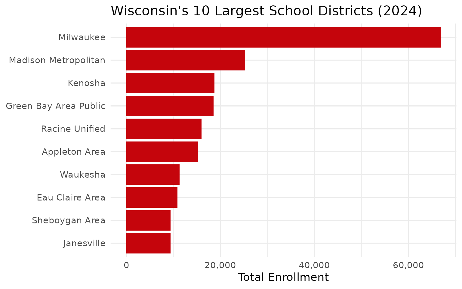
2. Milwaukee dominates the enrollment landscape
Milwaukee Public Schools is by far the largest district, serving nearly 67,000 students—more than the next two districts combined.
enr_2024 <- fetch_enr(2024, use_cache = TRUE)

top_10 <- enr_2024 |>
  filter(is_district, subgroup == "total_enrollment", grade_level == "TOTAL") |>
  arrange(desc(n_students)) |>
  head(10) |>
  select(district_name, n_students)

top_10
#>            district_name n_students
#> 1              Milwaukee      66864
#> 2   Madison Metropolitan      25247
#> 3                Kenosha      18719
#> 4  Green Bay Area Public      18579
#> 5         Racine Unified      15963
#> 6          Appleton Area      15230
#> 7               Waukesha      11318
#> 8        Eau Claire Area      10866
#> 9         Sheboygan Area       9427
#> 10            Janesville       9414
stopifnot(nrow(top_10) > 0)
top_10 |>
  mutate(district_name = forcats::fct_reorder(district_name, n_students)) |>
  ggplot(aes(x = n_students, y = district_name)) +
  geom_col(fill = "#C5050C") +
  scale_x_continuous(labels = scales::comma) +
  labs(
    title = "Wisconsin's 10 Largest School Districts (2024)",
    x = "Total Enrollment",
    y = NULL
  )
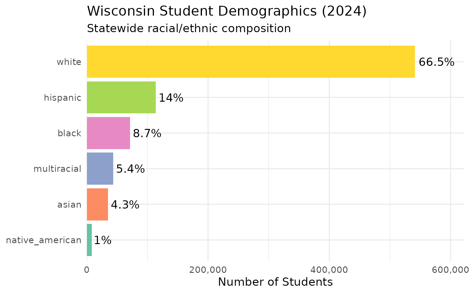
3. White students are two-thirds of statewide enrollment
Wisconsin remains predominantly white at 66.5%, but the student body is diversifying—Hispanic students now account for 14% and growing.
demographics <- enr_2024 |>
  filter(is_state, grade_level == "TOTAL",
         subgroup %in% c("hispanic", "white", "black", "asian", "multiracial", "native_american")) |>
  mutate(pct = round(pct * 100, 1)) |>
  select(subgroup, n_students, pct) |>
  arrange(desc(n_students))

demographics
#>          subgroup n_students  pct
#> 1           white     541411 66.5
#> 2        hispanic     114020 14.0
#> 3           black      71146  8.7
#> 4     multiracial      43621  5.4
#> 5           asian      34881  4.3
#> 6 native_american       8245  1.0
stopifnot(nrow(demographics) > 0)
demographics |>
  mutate(subgroup = forcats::fct_reorder(subgroup, n_students)) |>
  ggplot(aes(x = n_students, y = subgroup, fill = subgroup)) +
  geom_col(show.legend = FALSE) +
  geom_text(aes(label = paste0(pct, "%")), hjust = -0.1) +
  scale_x_continuous(labels = scales::comma, expand = expansion(mult = c(0, 0.15))) +
  scale_fill_brewer(palette = "Set2") +
  labs(
    title = "Wisconsin Student Demographics (2024)",
    subtitle = "Statewide racial/ethnic composition",
    x = "Number of Students",
    y = NULL
  )
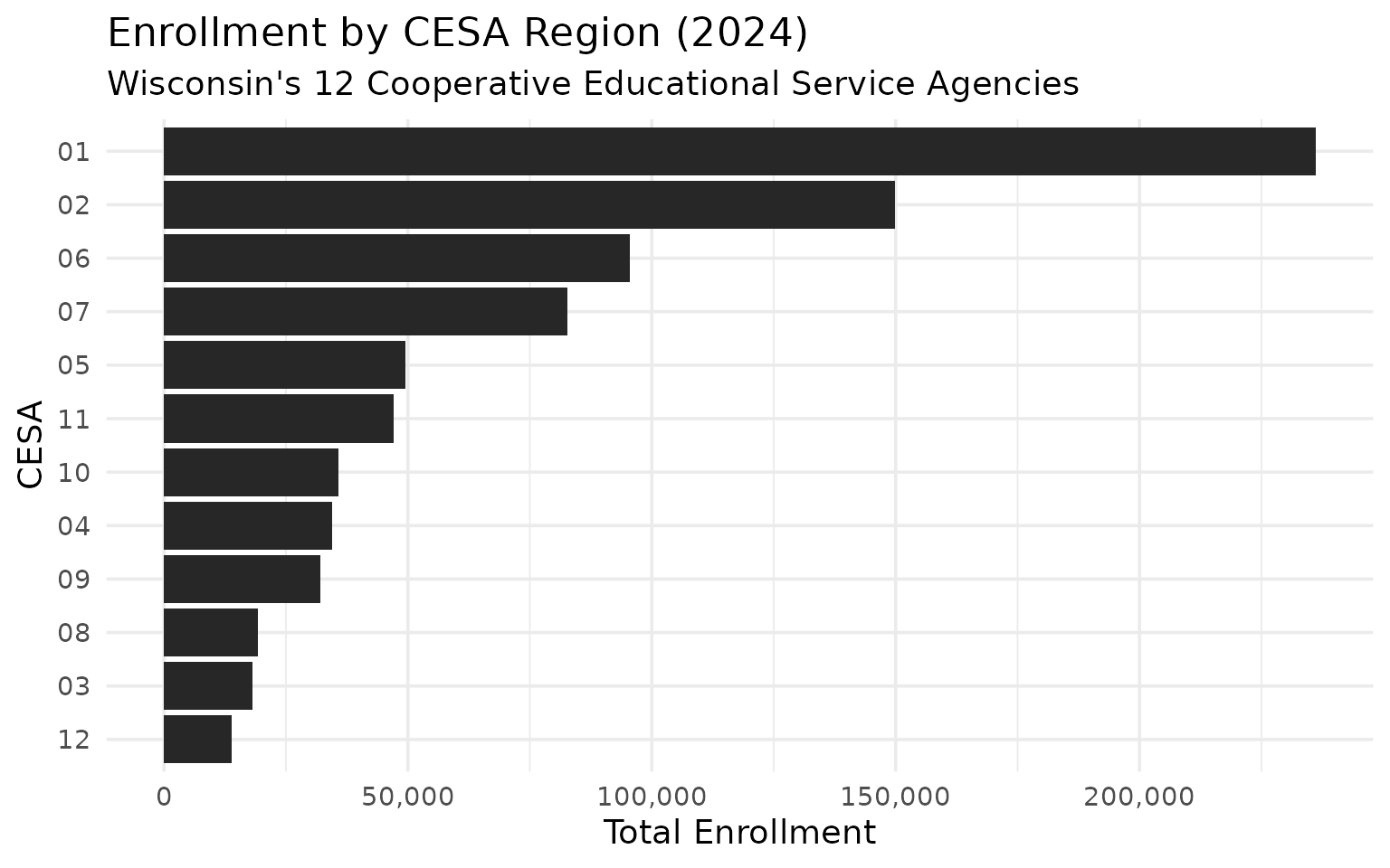
4. Wisconsin’s 12 CESAs organize regional services
Wisconsin divides into 12 Cooperative Educational Service Agencies (CESAs) that provide support services to districts. Enrollment varies widely by region.
cesa_totals <- enr_2024 |>
  filter(is_district, subgroup == "total_enrollment", grade_level == "TOTAL",
         !is.na(cesa)) |>
  group_by(cesa) |>
  summarize(
    n_districts = n_distinct(district_id),
    total_students = sum(n_students, na.rm = TRUE),
    .groups = "drop"
  ) |>
  arrange(desc(total_students))

cesa_totals
#> # A tibble: 12 × 3
#>    cesa  n_districts total_students
#>    <chr>       <int>          <dbl>
#>  1 01             66         236097
#>  2 02             78         149803
#>  3 06             39          95481
#>  4 07             38          82704
#>  5 05             36          49470
#>  6 11             39          47054
#>  7 10             29          35729
#>  8 04             26          34420
#>  9 09             22          32060
#> 10 08             27          19196
#> 11 03             31          18121
#> 12 12             18          13867
stopifnot(nrow(cesa_totals) > 0)
cesa_totals |>
  mutate(cesa = forcats::fct_reorder(as.factor(cesa), total_students)) |>
  ggplot(aes(x = total_students, y = cesa)) +
  geom_col(fill = "#282728") +
  scale_x_continuous(labels = scales::comma) +
  labs(
    title = "Enrollment by CESA Region (2024)",
    subtitle = "Wisconsin's 12 Cooperative Educational Service Agencies",
    x = "Total Enrollment",
    y = "CESA"
  )
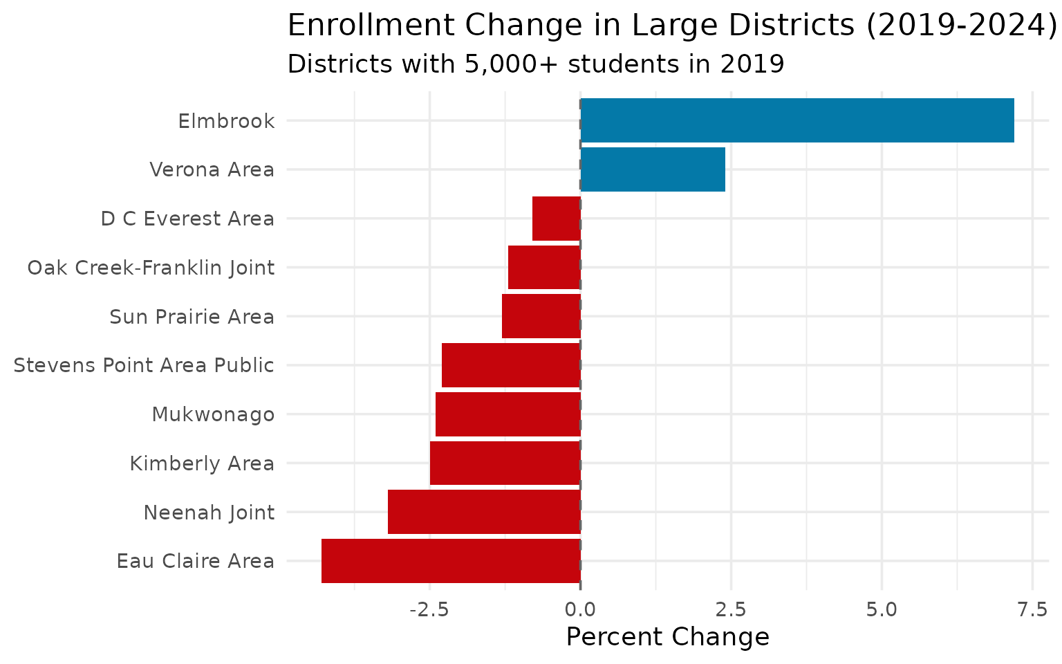
5. Most large districts are shrinking, with rare exceptions
Only Elmbrook and Verona bucked the trend among large districts—most lost students between 2019 and 2024, even in the suburbs.
growth <- enr |>
  filter(is_district, subgroup == "total_enrollment", grade_level == "TOTAL",
         end_year %in% c(2019, 2024)) |>
  group_by(district_id, district_name) |>
  filter(n() == 2) |>
  summarize(
    y2019 = n_students[end_year == 2019],
    y2024 = n_students[end_year == 2024],
    pct_change = round((y2024 / y2019 - 1) * 100, 1),
    .groups = "drop"
  ) |>
  filter(y2019 > 5000) |>
  arrange(desc(pct_change)) |>
  head(10)

growth
#> # A tibble: 10 × 5
#>    district_id district_name             y2019 y2024 pct_change
#>    <chr>       <chr>                     <dbl> <dbl>      <dbl>
#>  1 0714        Elmbrook                   7334  7863        7.2
#>  2 5901        Verona Area                5656  5794        2.4
#>  3 4970        D C Everest Area           6004  5954       -0.8
#>  4 4018        Oak Creek-Franklin Joint   6604  6527       -1.2
#>  5 5656        Sun Prairie Area           8521  8411       -1.3
#>  6 5607        Stevens Point Area Public  7144  6980       -2.3
#>  7 3822        Mukwonago                  5040  4918       -2.4
#>  8 2835        Kimberly Area              5190  5058       -2.5
#>  9 3892        Neenah Joint               6714  6497       -3.2
#> 10 1554        Eau Claire Area           11355 10866       -4.3
stopifnot(nrow(growth) > 0)
growth |>
  mutate(district_name = forcats::fct_reorder(district_name, pct_change)) |>
  ggplot(aes(x = pct_change, y = district_name, fill = pct_change > 0)) +
  geom_col(show.legend = FALSE) +
  geom_vline(xintercept = 0, linetype = "dashed", color = "gray40") +
  scale_fill_manual(values = c("TRUE" = "#0479A8", "FALSE" = "#C5050C")) +
  labs(
    title = "Enrollment Change in Large Districts (2019-2024)",
    subtitle = "Districts with 5,000+ students in 2019",
    x = "Percent Change",
    y = NULL
  )
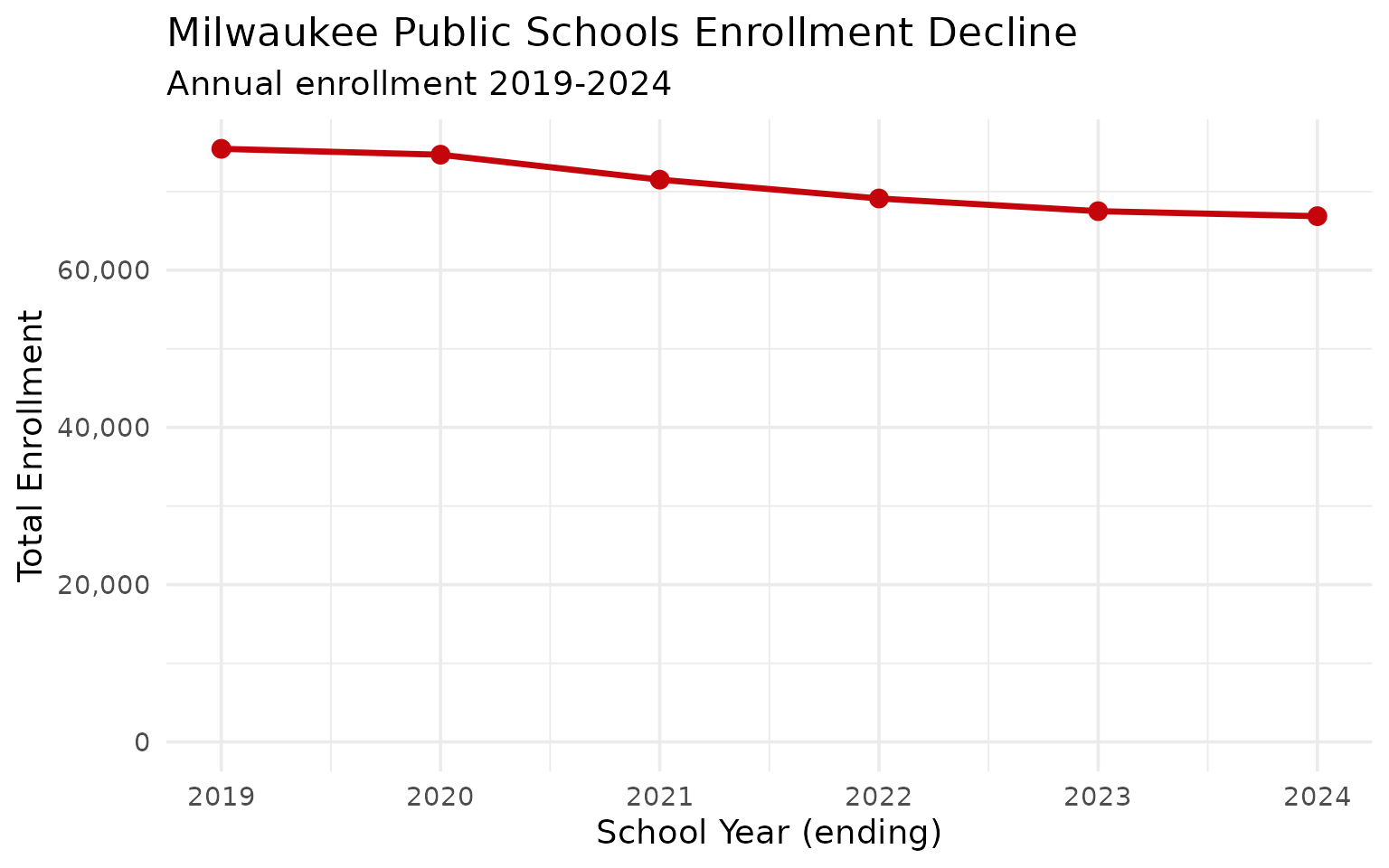
6. Milwaukee’s enrollment has declined significantly
Milwaukee Public Schools has lost thousands of students in recent years, driven by choice programs, charter schools, and population shifts.
milwaukee <- enr |>
  filter(is_district, subgroup == "total_enrollment", grade_level == "TOTAL",
         district_name == "Milwaukee")

milwaukee_summary <- milwaukee |>
  select(end_year, district_name, n_students) |>
  arrange(district_name, end_year)

milwaukee_summary
#>   end_year district_name n_students
#> 1     2019     Milwaukee      75431
#> 2     2020     Milwaukee      74683
#> 3     2021     Milwaukee      71510
#> 4     2022     Milwaukee      69115
#> 5     2023     Milwaukee      67500
#> 6     2024     Milwaukee      66864
stopifnot(nrow(milwaukee_summary) > 0)
milwaukee_summary |>
  filter(district_name == "Milwaukee") |>
  ggplot(aes(x = end_year, y = n_students)) +
  geom_line(linewidth = 1.2, color = "#C5050C") +
  geom_point(size = 3, color = "#C5050C") +
  scale_y_continuous(labels = scales::comma, limits = c(0, NA)) +
  labs(
    title = "Milwaukee Public Schools Enrollment Decline",
    subtitle = "Annual enrollment 2019-2024",
    x = "School Year (ending)",
    y = "Total Enrollment"
  )
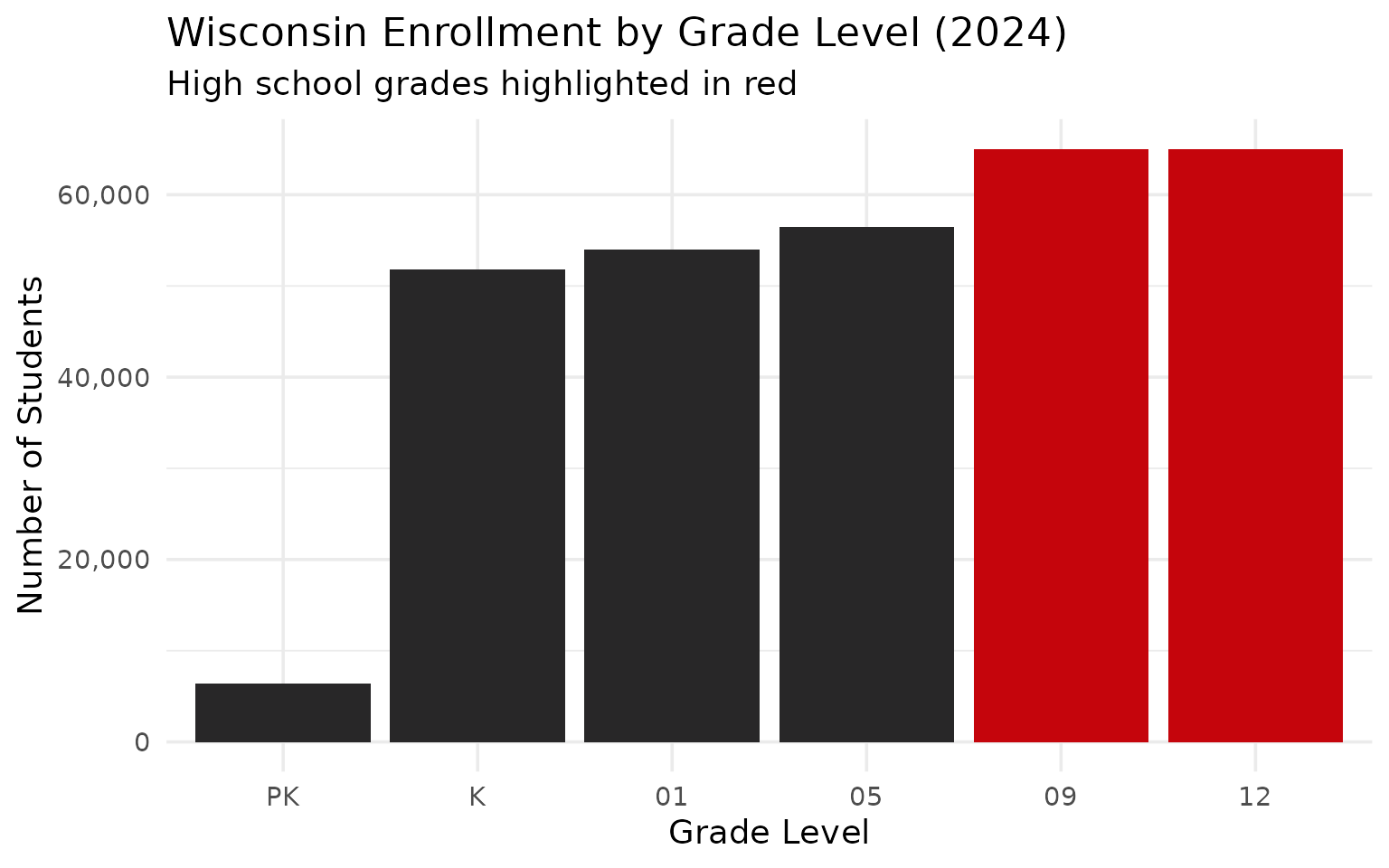
7. High school grades outpace elementary enrollment
Wisconsin enrolls more students in grades 9-12 than in early grades—a sign that high school retention is strong even as overall enrollment declines.
grade_breakdown <- enr_2024 |>
  filter(is_state, subgroup == "total_enrollment",
         grade_level %in% c("PK", "K", "01", "05", "09", "12")) |>
  select(grade_level, n_students) |>
  arrange(match(grade_level, c("PK", "K", "01", "05", "09", "12")))

grade_breakdown
#>   grade_level n_students
#> 1          PK       6363
#> 2           K      51787
#> 3          01      53983
#> 4          05      56459
#> 5          09      65035
#> 6          12      64957
stopifnot(nrow(grade_breakdown) > 0)
grade_breakdown |>
  mutate(grade_level = factor(grade_level, levels = c("PK", "K", "01", "05", "09", "12"))) |>
  ggplot(aes(x = grade_level, y = n_students, fill = grade_level %in% c("09", "12"))) +
  geom_col(show.legend = FALSE) +
  scale_y_continuous(labels = scales::comma) +
  scale_fill_manual(values = c("TRUE" = "#C5050C", "FALSE" = "#282728")) +
  labs(
    title = "Wisconsin Enrollment by Grade Level (2024)",
    subtitle = "High school grades highlighted in red",
    x = "Grade Level",
    y = "Number of Students"
  )
8. Rural dairy country districts are small but numerous
Wisconsin has hundreds of small rural districts, many in the state’s famous dairy farming regions. Most have fewer than 1,000 students.
size_distribution <- enr_2024 |>
  filter(is_district, subgroup == "total_enrollment", grade_level == "TOTAL") |>
  mutate(size_category = case_when(
    n_students < 500 ~ "Under 500",
    n_students < 1000 ~ "500-999",
    n_students < 2500 ~ "1,000-2,499",
    n_students < 5000 ~ "2,500-4,999",
    n_students < 10000 ~ "5,000-9,999",
    TRUE ~ "10,000+"
  )) |>
  mutate(size_category = factor(size_category,
    levels = c("Under 500", "500-999", "1,000-2,499", "2,500-4,999", "5,000-9,999", "10,000+"))) |>
  count(size_category) |>
  mutate(pct = round(n / sum(n) * 100, 1))

size_distribution
#>   size_category   n  pct
#> 1     Under 500 136 30.3
#> 2       500-999 124 27.6
#> 3   1,000-2,499 108 24.1
#> 4   2,500-4,999  50 11.1
#> 5   5,000-9,999  23  5.1
#> 6       10,000+   8  1.8
stopifnot(nrow(size_distribution) > 0)
size_distribution |>
  ggplot(aes(x = size_category, y = n, fill = size_category %in% c("Under 500", "500-999"))) +
  geom_col(show.legend = FALSE) +
  geom_text(aes(label = paste0(n, " (", pct, "%)")), vjust = -0.3, size = 3.5) +
  scale_fill_manual(values = c("TRUE" = "#C5050C", "FALSE" = "#282728")) +
  scale_y_continuous(expand = expansion(mult = c(0, 0.15))) +
  labs(
    title = "Wisconsin Districts by Size (2024)",
    subtitle = "Small rural districts (under 1,000 students) highlighted",
    x = "District Size Category",
    y = "Number of Districts"
  ) +
  theme(axis.text.x = element_text(angle = 45, hjust = 1))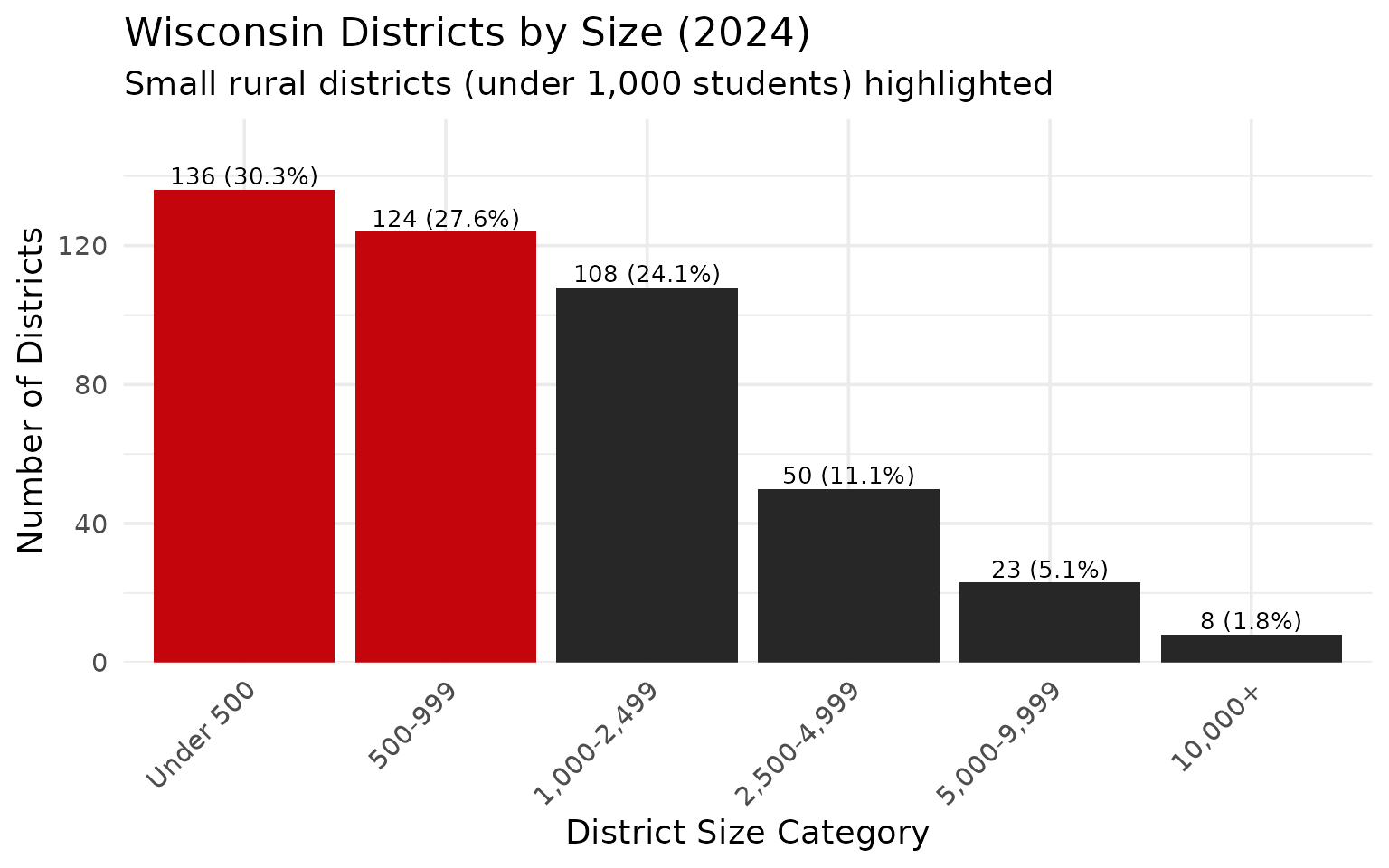
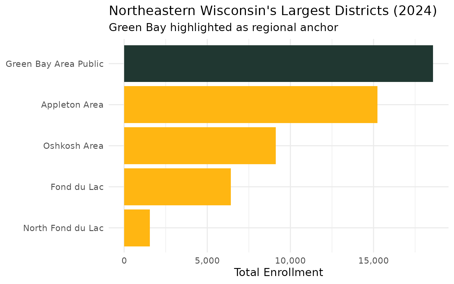
9. Green Bay anchors northeastern Wisconsin
Green Bay Area Public Schools is the largest district in northeastern Wisconsin, serving the region’s industrial and shipping hub.
fox_valley <- enr_2024 |>
  filter(is_district, subgroup == "total_enrollment", grade_level == "TOTAL",
         grepl("Green Bay|Appleton|Oshkosh|Fond du Lac", district_name, ignore.case = TRUE)) |>
  select(district_name, n_students) |>
  arrange(desc(n_students))

fox_valley
#>           district_name n_students
#> 1 Green Bay Area Public      18579
#> 2         Appleton Area      15230
#> 3          Oshkosh Area       9113
#> 4           Fond du Lac       6419
#> 5     North Fond du Lac       1555
stopifnot(nrow(fox_valley) > 0)
fox_valley |>
  mutate(district_name = forcats::fct_reorder(district_name, n_students)) |>
  ggplot(aes(x = n_students, y = district_name, fill = grepl("Green Bay", district_name))) +
  geom_col(show.legend = FALSE) +
  scale_x_continuous(labels = scales::comma) +
  scale_fill_manual(values = c("TRUE" = "#203731", "FALSE" = "#FFB612")) +
  labs(
    title = "Northeastern Wisconsin's Largest Districts (2024)",
    subtitle = "Green Bay highlighted as regional anchor",
    x = "Total Enrollment",
    y = NULL
  )
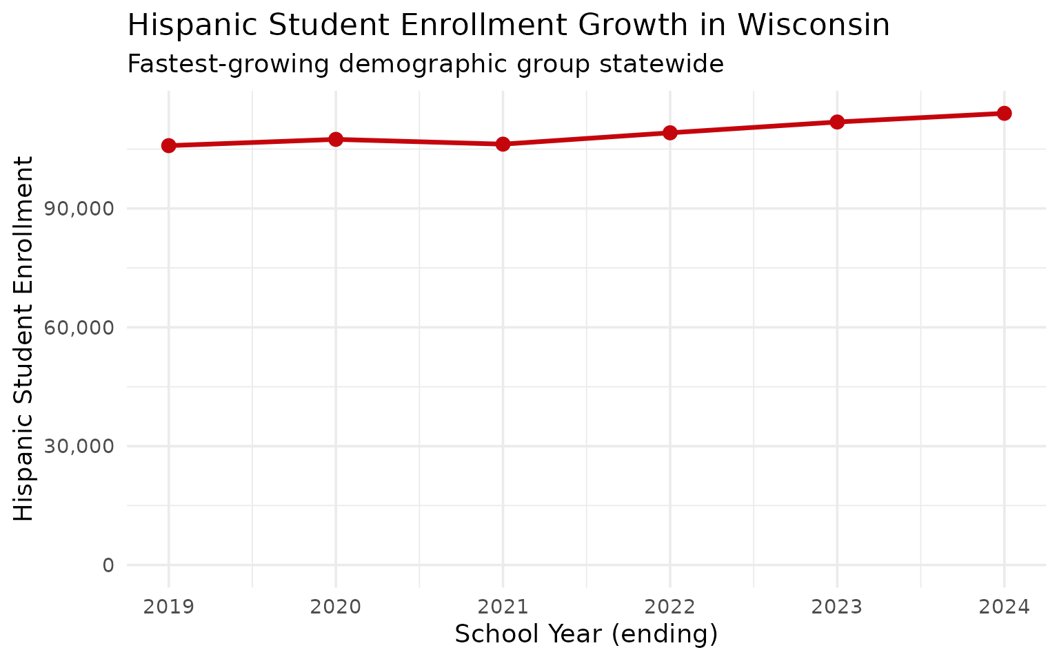
10. Hispanic enrollment is growing statewide
Hispanic students are the fastest-growing demographic group in Wisconsin, particularly in southeastern Wisconsin and agricultural communities.
hispanic_trend <- enr |>
  filter(is_state, grade_level == "TOTAL", subgroup == "hispanic") |>
  select(end_year, n_students, pct) |>
  mutate(pct = round(pct * 100, 1))

hispanic_trend
#>   end_year n_students  pct
#> 1     2019     105863 12.3
#> 2     2020     107448 12.6
#> 3     2021     106239 12.8
#> 4     2022     109106 13.2
#> 5     2023     111830 13.6
#> 6     2024     114020 14.0
stopifnot(nrow(hispanic_trend) > 0)
hispanic_trend |>
  ggplot(aes(x = end_year, y = n_students)) +
  geom_line(linewidth = 1.2, color = "#C5050C") +
  geom_point(size = 3, color = "#C5050C") +
  scale_y_continuous(labels = scales::comma, limits = c(0, NA)) +
  labs(
    title = "Hispanic Student Enrollment Growth in Wisconsin",
    subtitle = "Fastest-growing demographic group statewide",
    x = "School Year (ending)",
    y = "Hispanic Student Enrollment"
  )
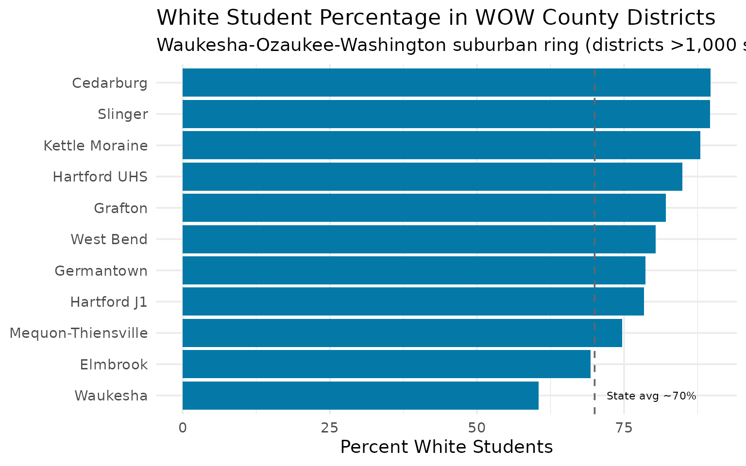
11. The WOW Counties: Suburban Milwaukee’s Demographic Mix
The WOW counties (Waukesha, Ozaukee, Washington) form an affluent suburban ring around Milwaukee with distinct demographic profiles—higher percentages of white students than the statewide average.
# Identify WOW-area districts by name patterns
wow_districts <- enr_2024 |>
  filter(is_district, grade_level == "TOTAL",
         subgroup %in% c("total_enrollment", "white")) |>
  select(district_name, subgroup, n_students) |>
  pivot_wider(names_from = subgroup, values_from = n_students) |>
  filter(grepl("Waukesha|Germantown|Cedarburg|Mequon|Hartford|West Bend|Grafton|Slinger|Elmbrook|Kettle Moraine",
               district_name, ignore.case = TRUE)) |>
  mutate(pct_white = round(white / total_enrollment * 100, 1)) |>
  filter(total_enrollment > 1000) |>
  arrange(desc(pct_white))

wow_districts
#> # A tibble: 11 × 4
#>    district_name      total_enrollment white pct_white
#>    <chr>                         <dbl> <dbl>     <dbl>
#>  1 Cedarburg                      3101  2781      89.7
#>  2 Slinger                        3271  2932      89.6
#>  3 Kettle Moraine                 3421  3010      88
#>  4 Hartford UHS                   1364  1158      84.9
#>  5 Grafton                        2132  1750      82.1
#>  6 West Bend                      5591  4495      80.4
#>  7 Germantown                     3816  2999      78.6
#>  8 Hartford J1                    1429  1120      78.4
#>  9 Mequon-Thiensville             3570  2667      74.7
#> 10 Elmbrook                       7863  5452      69.3
#> 11 Waukesha                      11318  6853      60.5
stopifnot(nrow(wow_districts) > 0)
wow_districts |>
  mutate(district_name = forcats::fct_reorder(district_name, pct_white)) |>
  ggplot(aes(x = pct_white, y = district_name)) +
  geom_col(fill = "#0479A8") +
  geom_vline(xintercept = 70, linetype = "dashed", color = "gray40") +
  annotate("text", x = 72, y = 1, label = "State avg ~70%", hjust = 0, size = 3) +
  labs(
    title = "White Student Percentage in WOW County Districts",
    subtitle = "Waukesha-Ozaukee-Washington suburban ring (districts >1,000 students)",
    x = "Percent White Students",
    y = NULL
  )
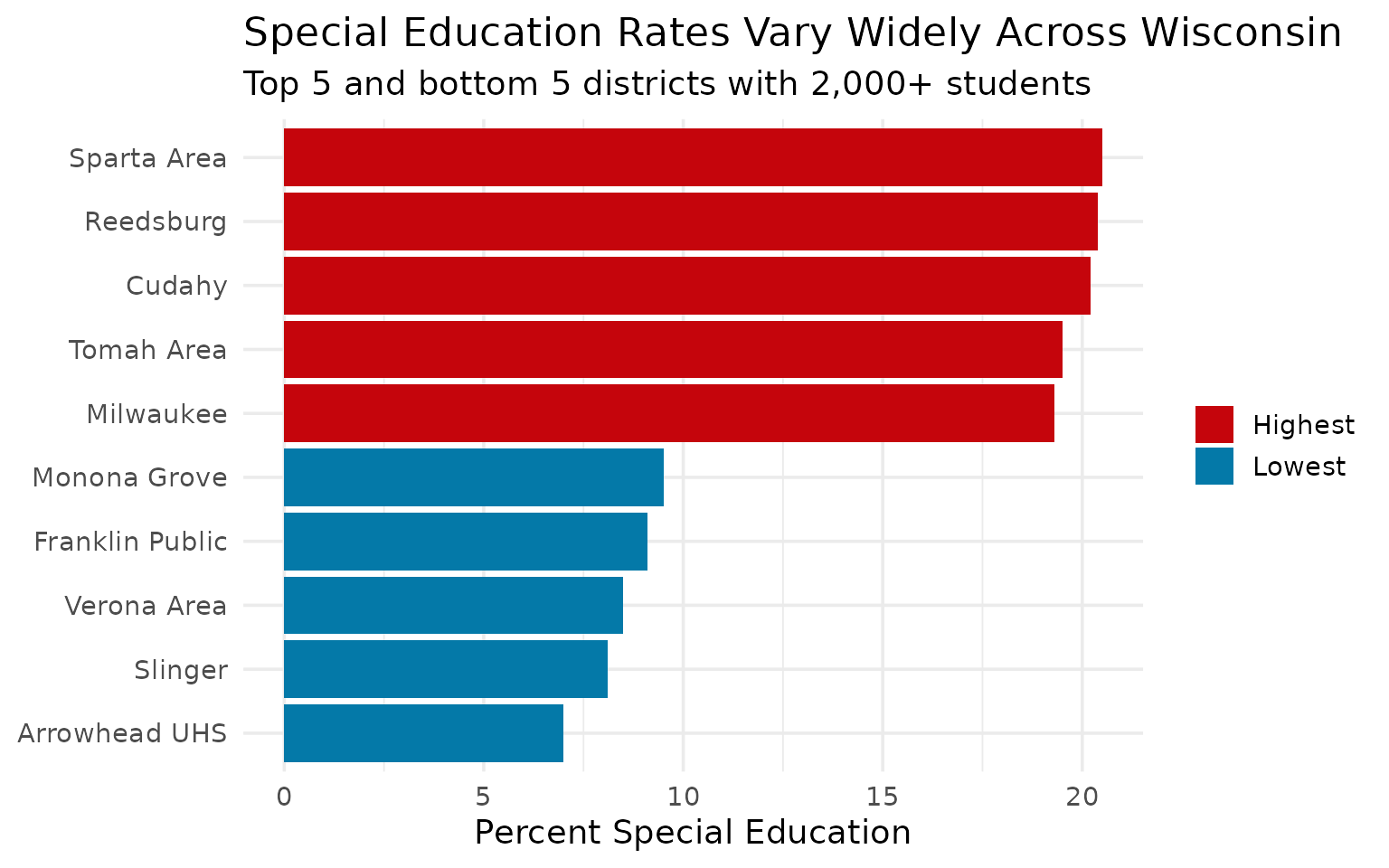
12. Special Education Varies by Region
Special education rates differ markedly across Wisconsin, with some districts serving twice the proportion of students with disabilities as others.
sped_rates <- enr_2024 |>
  filter(is_district, grade_level == "TOTAL",
         subgroup %in% c("total_enrollment", "special_ed")) |>
  select(district_name, subgroup, n_students) |>
  pivot_wider(names_from = subgroup, values_from = n_students) |>
  filter(total_enrollment > 2000) |>
  mutate(pct_sped = round(special_ed / total_enrollment * 100, 1)) |>
  arrange(desc(pct_sped))

sped_summary <- bind_rows(
  sped_rates |> head(5) |> mutate(group = "Highest"),
  sped_rates |> tail(5) |> mutate(group = "Lowest")
)

sped_summary
#> # A tibble: 10 × 5
#>    district_name   total_enrollment special_ed pct_sped group
#>    <chr>                      <dbl>      <dbl>    <dbl> <chr>
#>  1 Sparta Area                 2794        573     20.5 Highest
#>  2 Reedsburg                   2597        529     20.4 Highest
#>  3 Cudahy                      2054        415     20.2 Highest
#>  4 Tomah Area                  3096        603     19.5 Highest
#>  5 Milwaukee                  66864      12924     19.3 Highest
#>  6 Monona Grove                3696        352      9.5 Lowest
#>  7 Franklin Public             4721        428      9.1 Lowest
#>  8 Verona Area                 5794        491      8.5 Lowest
#>  9 Slinger                     3271        265      8.1 Lowest
#> 10 Arrowhead UHS               2038        143      7   Lowest
stopifnot(nrow(sped_summary) > 0)
sped_summary |>
  mutate(district_name = forcats::fct_reorder(district_name, pct_sped)) |>
  ggplot(aes(x = pct_sped, y = district_name, fill = group)) +
  geom_col(show.legend = TRUE) +
  scale_fill_manual(values = c("Highest" = "#C5050C", "Lowest" = "#0479A8")) +
  labs(
    title = "Special Education Rates Vary Widely Across Wisconsin",
    subtitle = "Top 5 and bottom 5 districts with 2,000+ students",
    x = "Percent Special Education",
    y = NULL,
    fill = NULL
  )
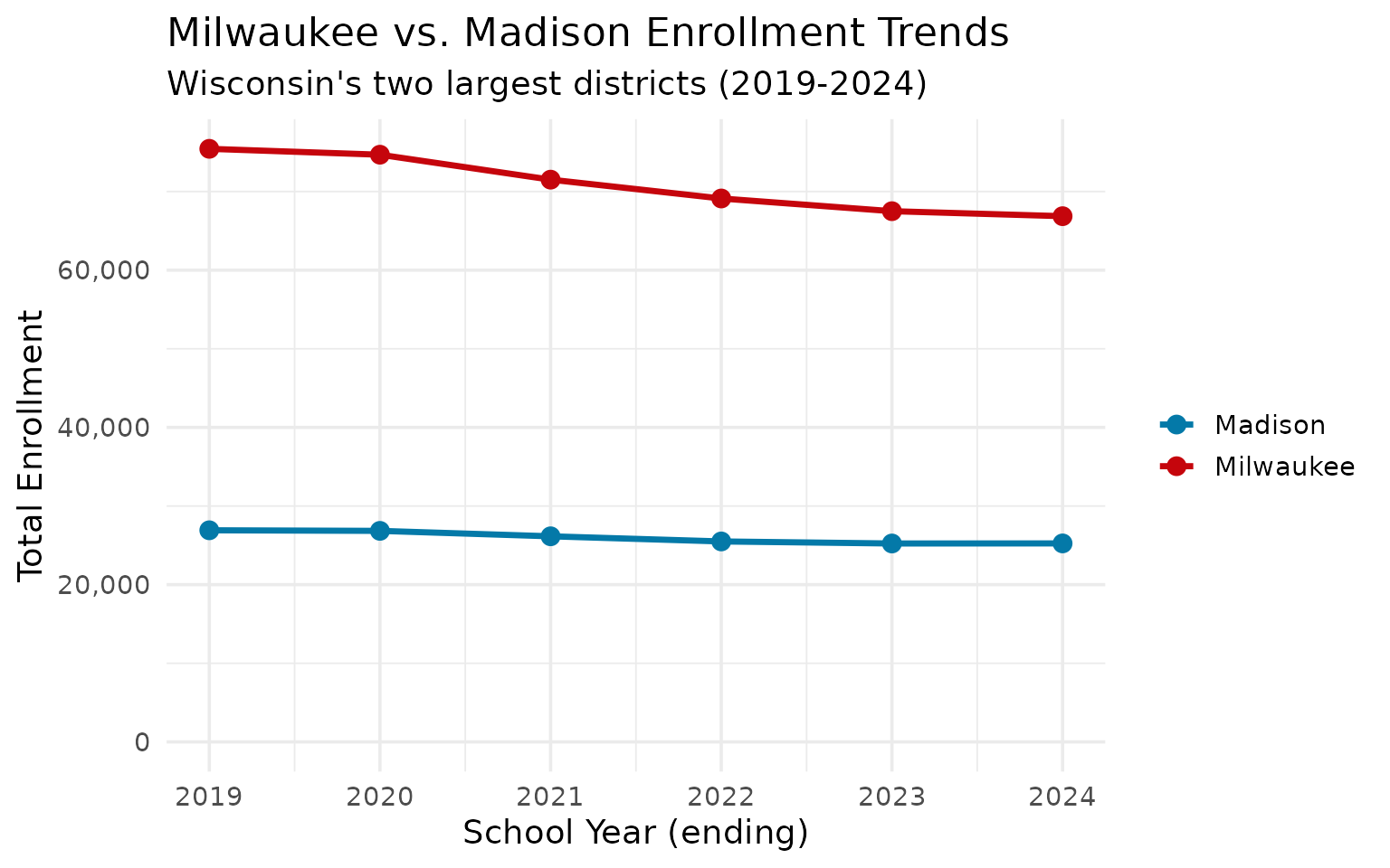
13. Madison vs. Milwaukee: A Tale of Two Cities
Wisconsin’s two largest cities are both losing students, but Milwaukee’s decline is far steeper—Milwaukee’s losses dwarf Madison’s over the same period.
two_cities <- enr |>
  filter(is_district, subgroup == "total_enrollment", grade_level == "TOTAL",
         grepl("^Milwaukee$|Madison Metropolitan", district_name)) |>
  select(end_year, district_name, n_students)

two_cities
#>    end_year        district_name n_students
#> 1      2019 Madison Metropolitan      26917
#> 2      2019            Milwaukee      75431
#> 3      2020 Madison Metropolitan      26842
#> 4      2020            Milwaukee      74683
#> 5      2021 Madison Metropolitan      26151
#> 6      2021            Milwaukee      71510
#> 7      2022 Madison Metropolitan      25497
#> 8      2022            Milwaukee      69115
#> 9      2023 Madison Metropolitan      25237
#> 10     2023            Milwaukee      67500
#> 11     2024 Madison Metropolitan      25247
#> 12     2024            Milwaukee      66864
stopifnot(nrow(two_cities) > 0)
two_cities |>
  mutate(city = ifelse(grepl("Milwaukee", district_name), "Milwaukee", "Madison")) |>
  ggplot(aes(x = end_year, y = n_students, color = city)) +
  geom_line(linewidth = 1.2) +
  geom_point(size = 3) +
  scale_y_continuous(labels = scales::comma, limits = c(0, NA)) +
  scale_color_manual(values = c("Milwaukee" = "#C5050C", "Madison" = "#0479A8")) +
  labs(
    title = "Milwaukee vs. Madison Enrollment Trends",
    subtitle = "Wisconsin's two largest districts (2019-2024)",
    x = "School Year (ending)",
    y = "Total Enrollment",
    color = NULL
  )
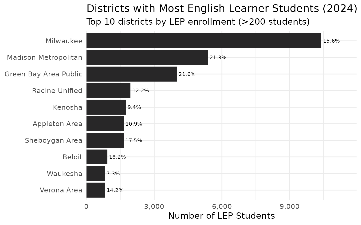
14. English Learners Concentrated in Urban Areas
Limited English Proficiency (LEP) students are heavily concentrated in a handful of urban districts, with Milwaukee and Madison serving the vast majority.
lep_districts <- enr_2024 |>
  filter(is_district, grade_level == "TOTAL",
         subgroup %in% c("total_enrollment", "lep")) |>
  select(district_name, subgroup, n_students) |>
  pivot_wider(names_from = subgroup, values_from = n_students) |>
  filter(lep > 200) |>
  mutate(pct_lep = round(lep / total_enrollment * 100, 1)) |>
  arrange(desc(lep)) |>
  head(10)

lep_districts
#> # A tibble: 10 × 4
#>    district_name         total_enrollment   lep pct_lep
#>    <chr>                            <dbl> <dbl>   <dbl>
#>  1 Milwaukee                        66864 10404    15.6
#>  2 Madison Metropolitan             25247  5377    21.3
#>  3 Green Bay Area Public            18579  4011    21.6
#>  4 Racine Unified                   15963  1953    12.2
#>  5 Kenosha                          18719  1760     9.4
#>  6 Appleton Area                    15230  1653    10.9
#>  7 Sheboygan Area                    9427  1646    17.5
#>  8 Beloit                            5098   926    18.2
#>  9 Waukesha                         11318   830     7.3
#> 10 Verona Area                       5794   822    14.2
stopifnot(nrow(lep_districts) > 0)
lep_districts |>
  mutate(district_name = forcats::fct_reorder(district_name, lep)) |>
  ggplot(aes(x = lep, y = district_name)) +
  geom_col(fill = "#282728") +
  geom_text(aes(label = paste0(pct_lep, "%")), hjust = -0.1, size = 3) +
  scale_x_continuous(labels = scales::comma, expand = expansion(mult = c(0, 0.15))) +
  labs(
    title = "Districts with Most English Learner Students (2024)",
    subtitle = "Top 10 districts by LEP enrollment (>200 students)",
    x = "Number of LEP Students",
    y = NULL
  )
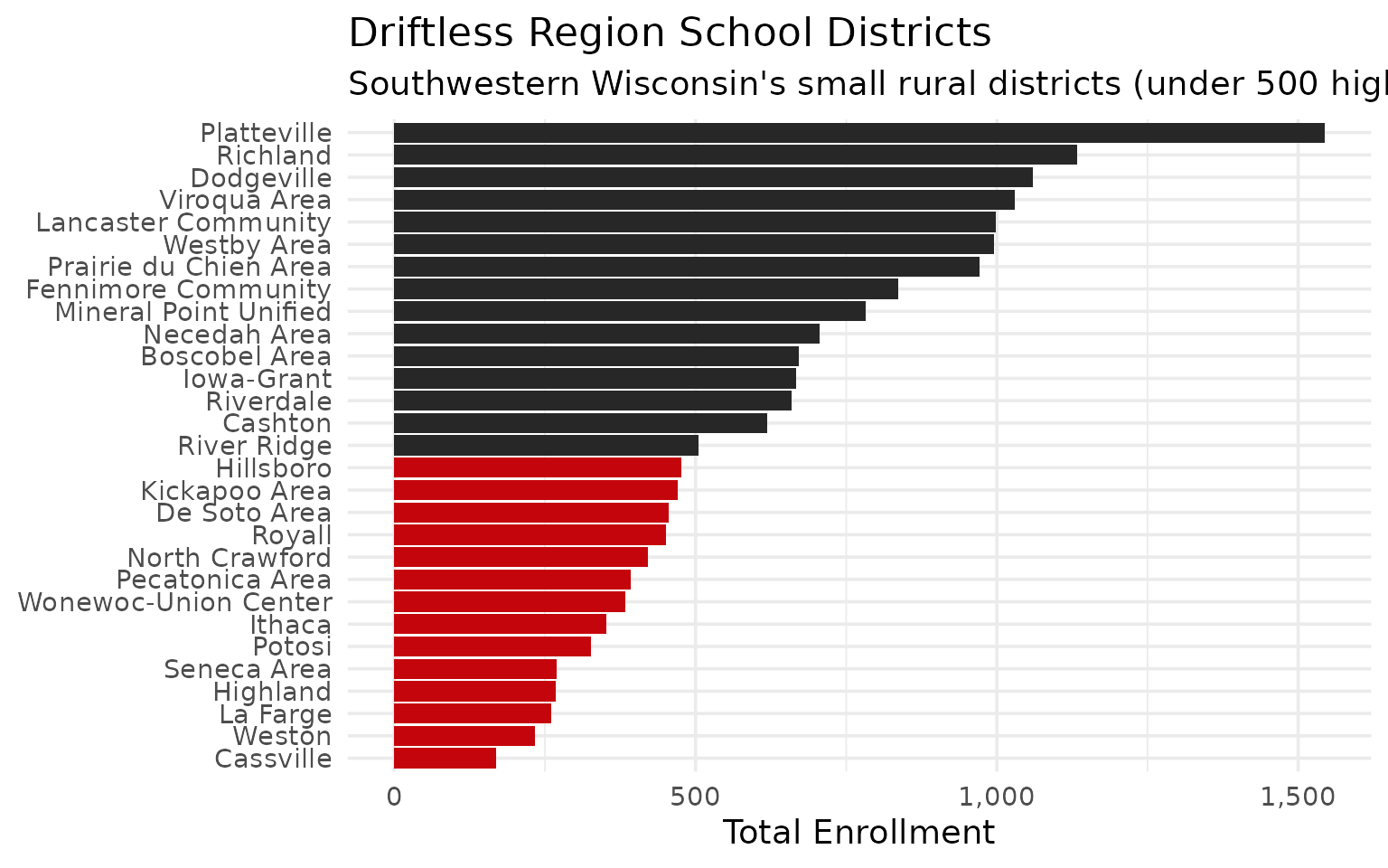
15. The Driftless Region’s Small School Districts
Southwestern Wisconsin’s Driftless Area—unglaciated terrain known for dairy farms and winding valleys—is home to dozens of tiny school districts.
# Driftless region includes Crawford, Grant, Iowa, Lafayette, Richland, Vernon, and parts of others
driftless_districts <- enr_2024 |>
  filter(is_district, subgroup == "total_enrollment", grade_level == "TOTAL",
         grepl("Prairie du Chien|Richland|Viroqua|Kickapoo|Westby|Cashton|La Farge|Hillsboro|Wonewoc|Necedah|Royall|Boscobel|Lancaster|Platteville|Fennimore|Potosi|Cassville|Seneca|River Ridge|Ithaca|Weston|De Soto|North Crawford|Riverdale|Pecatonica|Iowa-Grant|Highland|Mineral Point|Dodgeville",
               district_name, ignore.case = TRUE)) |>
  select(district_name, n_students) |>
  arrange(n_students)

driftless_districts
#>            district_name n_students
#> 1              Cassville        169
#> 2                 Weston        233
#> 3               La Farge        260
#> 4               Highland        268
#> 5            Seneca Area        270
#> 6                 Potosi        327
#> 7                 Ithaca        352
#> 8   Wonewoc-Union Center        384
#> 9        Pecatonica Area        393
#> 10        North Crawford        421
#> 11                Royall        451
#> 12          De Soto Area        455
#> 13         Kickapoo Area        471
#> 14             Hillsboro        477
#> 15           River Ridge        505
#> 16               Cashton        619
#> 17             Riverdale        660
#> 18            Iowa-Grant        667
#> 19         Boscobel Area        672
#> 20          Necedah Area        706
#> 21 Mineral Point Unified        782
#> 22   Fennimore Community        836
#> 23 Prairie du Chien Area        971
#> 24           Westby Area        995
#> 25   Lancaster Community        999
#> 26          Viroqua Area       1030
#> 27            Dodgeville       1060
#> 28              Richland       1133
#> 29           Platteville       1544
stopifnot(nrow(driftless_districts) > 0)
driftless_districts |>
  mutate(district_name = forcats::fct_reorder(district_name, n_students)) |>
  ggplot(aes(x = n_students, y = district_name,
             fill = n_students < 500)) +
  geom_col(show.legend = FALSE) +
  scale_x_continuous(labels = scales::comma) +
  scale_fill_manual(values = c("TRUE" = "#C5050C", "FALSE" = "#282728")) +
  labs(
    title = "Driftless Region School Districts",
    subtitle = "Southwestern Wisconsin's small rural districts (under 500 highlighted)",
    x = "Total Enrollment",
    y = NULL
  )
Summary
Wisconsin’s school enrollment data reveals:
- Statewide decline: Wisconsin has lost nearly 45,000 students since 2019, a trend that accelerated during and after COVID
- Predominantly white: White students make up two-thirds of statewide enrollment, but diversity is increasing
- Broad-based decline: Most large districts are shrinking, with only a few suburban exceptions like Elmbrook and Verona
- Small district heritage: Hundreds of tiny rural districts serve dairy country communities
- Demographic change: Hispanic enrollment is growing, reshaping the state’s student population
- Suburban demographics: WOW counties have distinct demographic profiles from urban cores
- Service variation: Special education and English learner rates vary significantly by region
- Two cities decline: Both Madison and Milwaukee are losing students, but Milwaukee’s decline is far steeper
These patterns shape education policy across the Badger State.
Data sourced from the Wisconsin Department of Public Instruction.
sessionInfo()
#> R version 4.5.2 (2025-10-31)
#> Platform: x86_64-pc-linux-gnu
#> Running under: Ubuntu 24.04.3 LTS
#>
#> Matrix products: default
#> BLAS:   /usr/lib/x86_64-linux-gnu/openblas-pthread/libblas.so.3
#> LAPACK: /usr/lib/x86_64-linux-gnu/openblas-pthread/libopenblasp-r0.3.26.so;  LAPACK version 3.12.0
#>
#> locale:
#>  [1] LC_CTYPE=C.UTF-8       LC_NUMERIC=C           LC_TIME=C.UTF-8
#>  [4] LC_COLLATE=C.UTF-8     LC_MONETARY=C.UTF-8    LC_MESSAGES=C.UTF-8
#>  [7] LC_PAPER=C.UTF-8       LC_NAME=C              LC_ADDRESS=C
#> [10] LC_TELEPHONE=C         LC_MEASUREMENT=C.UTF-8 LC_IDENTIFICATION=C
#>
#> time zone: UTC
#> tzcode source: system (glibc)
#>
#> attached base packages:
#> [1] stats     graphics  grDevices utils     datasets  methods   base
#>
#> other attached packages:
#> [1] ggplot2_4.0.2      tidyr_1.3.2        dplyr_1.2.0        wischooldata_0.1.0
#>
#> loaded via a namespace (and not attached):
#>  [1] utf8_1.2.6         rappdirs_0.3.4     sass_0.4.10        generics_0.1.4
#>  [5] hms_1.1.4          digest_0.6.39      magrittr_2.0.4     evaluate_1.0.5
#>  [9] grid_4.5.2         RColorBrewer_1.1-3 fastmap_1.2.0      jsonlite_2.0.0
#> [13] httr_1.4.8         purrr_1.2.1        scales_1.4.0       codetools_0.2-20
#> [17] textshaping_1.0.4  jquerylib_0.1.4    cli_3.6.5          rlang_1.1.7
#> [21] crayon_1.5.3       bit64_4.6.0-1      withr_3.0.2        cachem_1.1.0
#> [25] yaml_2.3.12        tools_4.5.2        parallel_4.5.2     tzdb_0.5.0
#> [29] forcats_1.0.1      curl_7.0.0         vctrs_0.7.1        R6_2.6.1
#> [33] lifecycle_1.0.5    fs_1.6.6           bit_4.6.0          vroom_1.7.0
#> [37] ragg_1.5.0         pkgconfig_2.0.3    desc_1.4.3         pkgdown_2.2.0
#> [41] pillar_1.11.1      bslib_0.10.0       gtable_0.3.6       glue_1.8.0
#> [45] systemfonts_1.3.1  xfun_0.56          tibble_3.3.1       tidyselect_1.2.1
#> [49] knitr_1.51         farver_2.1.2       htmltools_0.5.9    rmarkdown_2.30
#> [53] labeling_0.4.3     readr_2.2.0        compiler_4.5.2     S7_0.2.1