library(azschooldata)
library(dplyr)
library(tidyr)
library(ggplot2)

theme_set(theme_minimal(base_size = 14))
This vignette explores Arizona’s public school enrollment data from the Arizona Department of Education.
Data available: 2018, 2019, 2024, 2025, and 2026. Years 2020-2023 are not available as automated Excel downloads due to Cloudflare protection.
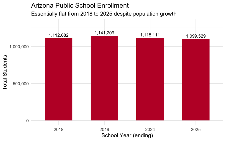
1. Arizona enrollment fell despite population boom
While Arizona’s population grew significantly from 2018-2025, public school enrollment actually declined - from 1.11 million to 1.10 million students. Enrollment peaked in 2019 (1.14M) then fell 3.7% by 2025. This suggests more families are choosing private schools, homeschooling, or leaving the public system.
enr <- fetch_enr_multi(c(2018, 2019, 2024, 2025), use_cache = TRUE)

state_enr <- enr |>
  filter(is_state,
         subgroup == "total_enrollment", grade_level == "TOTAL") |>
  select(end_year, n_students) |>
  mutate(change = n_students - lag(n_students),
         pct_change = round(change / lag(n_students) * 100, 1))
stopifnot(nrow(state_enr) > 0)
state_enr
#>   end_year n_students change pct_change
#> 1     2018    1112682     NA         NA
#> 2     2019    1141209  28527        2.6
#> 3     2024    1115111 -26098       -2.3
#> 4     2025    1099529 -15582       -1.4
state_enr_chart <- enr |>
  filter(is_state,
         subgroup == "total_enrollment", grade_level == "TOTAL")
stopifnot(nrow(state_enr_chart) > 0)
state_enr_chart |>
  ggplot(aes(x = factor(end_year), y = n_students)) +
  geom_col(fill = "#BF0A30", width = 0.6) +
  geom_text(aes(label = scales::comma(n_students)), vjust = -0.5, size = 4) +
  scale_y_continuous(labels = scales::comma, limits = c(0, 1300000)) +
  labs(
    title = "Arizona Public School Enrollment",
    subtitle = "Essentially flat from 2018 to 2025 despite population growth",
    x = "School Year (ending)",
    y = "Total Students"
  )
2. Hispanic students now 49% of Arizona schools
Hispanic students grew from 45.7% in 2018 to 48.8% in 2025, while White students declined from 38.0% to 32.9%. Arizona’s schools are becoming increasingly diverse.
demographics <- enr |>
  filter(is_state, grade_level == "TOTAL",
         subgroup %in% c("hispanic", "white", "black", "asian",
                         "native_american", "multiracial", "total_enrollment")) |>
  group_by(end_year) |>
  mutate(pct = round(n_students / n_students[subgroup == "total_enrollment"] * 100, 1)) |>
  filter(subgroup != "total_enrollment")
stopifnot(nrow(demographics) > 0)

demographics |>
  select(end_year, subgroup, n_students, pct) |>
  arrange(end_year, desc(n_students))
#> # A tibble: 24 × 4
#> # Groups:   end_year [4]
#>    end_year subgroup        n_students   pct
#>       <dbl> <chr>                <dbl> <dbl>
#>  1     2018 hispanic            508121  45.7
#>  2     2018 white               422414  38
#>  3     2018 black                58875   5.3
#>  4     2018 native_american      48579   4.4
#>  5     2018 multiracial          33218   3
#>  6     2018 asian                31283   2.8
#>  7     2019 hispanic            520535  45.6
#>  8     2019 white               430623  37.7
#>  9     2019 black                61568   5.4
#> 10     2019 native_american      49650   4.4
#> # ℹ 14 more rows
demo_2025 <- demographics |>
  filter(end_year == 2025) |>
  mutate(subgroup = factor(subgroup, levels = c("hispanic", "white", "black",
                                                 "native_american", "asian", "multiracial")))
stopifnot(nrow(demo_2025) > 0)
demo_2025 |>
  ggplot(aes(x = reorder(subgroup, -n_students), y = n_students, fill = subgroup)) +
  geom_col() +
  scale_fill_brewer(palette = "Set2") +
  scale_y_continuous(labels = scales::comma) +
  labs(
    title = "Arizona School Enrollment by Race/Ethnicity (2025)",
    subtitle = "Hispanic students are the largest group at 49%",
    x = NULL,
    y = "Number of Students"
  ) +
  theme(legend.position = "none",
        axis.text.x = element_text(angle = 45, hjust = 1))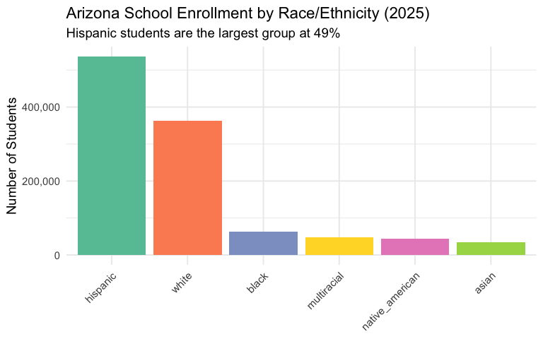
3. Queen Creek doubled in size while Mesa lost 7,100 students
Queen Creek Unified grew 112% (from 7,095 to 15,034 students) as new subdivisions opened in the southeast Valley. Meanwhile, Mesa Unified - the state’s largest district - lost 7,156 students (-11.4%).
growth <- enr |>
  filter(is_district,
         subgroup == "total_enrollment", grade_level == "TOTAL") |>
  group_by(end_year, district_name) |>
  summarize(n_students = sum(n_students, na.rm = TRUE), .groups = "drop") |>
  pivot_wider(names_from = end_year, values_from = n_students,
              names_prefix = "y") |>
  filter(!is.na(y2018), !is.na(y2025), y2018 >= 1000) |>
  mutate(change = y2025 - y2018,
         pct_change = round((y2025 / y2018 - 1) * 100, 1)) |>
  arrange(desc(change))
stopifnot(nrow(growth) > 0)

growth |>
  select(district_name, y2018, y2025, change, pct_change) |>
  head(10)
#> # A tibble: 10 × 5
#>    district_name                           y2018 y2025 change pct_change
#>    <chr>                                   <dbl> <dbl>  <dbl>      <dbl>
#>  1 Queen Creek Unified District             7095 15034   7939      112.
#>  2 American Leadership Academy, Inc.        7904 15266   7362       93.1
#>  3 Maricopa Unified School District         6661  9504   2843       42.7
#>  4 Tolleson Union High School District     11152 13901   2749       24.7
#>  5 Leman Academy of Excellence, Inc.        2042  4592   2550      125.
#>  6 Agua Fria Union High School District     7766 10074   2308       29.7
#>  7 American Virtual Academy                 4227  6289   2062       48.8
#>  8 Saddle Mountain Unified School District  1630  3256   1626       99.8
#>  9 Buckeye Union High School District       4014  5634   1620       40.4
#> 10 GAR, LLC dba Student Choice High School  1054  2370   1316      125.
growth_top10 <- growth |>
  head(10) |>
  mutate(district_name = gsub(" District.*$| Unified.*$", "", district_name))
stopifnot(nrow(growth_top10) > 0)
growth_top10 |>
  ggplot(aes(x = reorder(district_name, change), y = change, fill = change > 0)) +
  geom_col() +
  coord_flip() +
  scale_fill_manual(values = c("TRUE" = "#2E8B57", "FALSE" = "#CD5C5C")) +
  scale_y_continuous(labels = scales::comma) +
  labs(
    title = "Top 10 Fastest Growing Districts (2018-2025)",
    subtitle = "Queen Creek added 7,939 students (+112%)",
    x = NULL,
    y = "Change in Enrollment"
  ) +
  theme(legend.position = "none")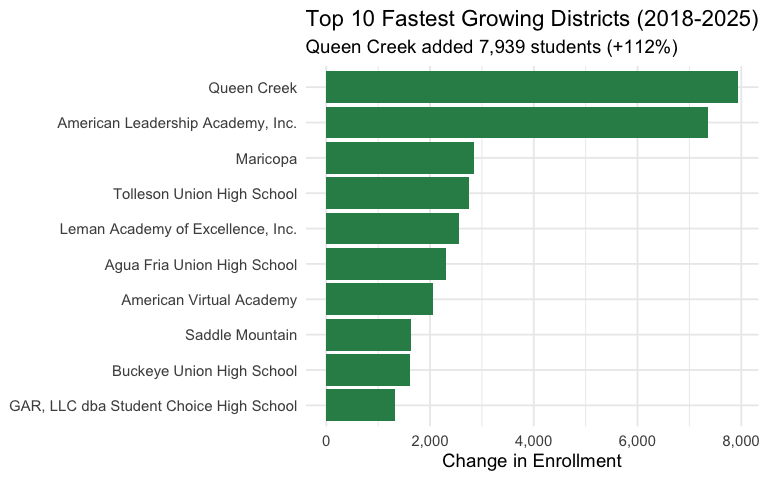
4. Mesa, Tucson, and Paradise Valley lead enrollment losses
The three largest enrollment declines in Arizona are all in established urban districts: Mesa (-7,156), Tucson (-5,265), and Paradise Valley (-5,081). These districts face competition from charters and demographic shifts.
growth |>
  arrange(change) |>
  select(district_name, y2018, y2025, change, pct_change) |>
  head(10)
#> # A tibble: 10 × 5
#>    district_name                         y2018 y2025 change pct_change
#>    <chr>                                 <dbl> <dbl>  <dbl>      <dbl>
#>  1 Mesa Unified District                 62756 55600  -7156      -11.4
#>  2 Tucson Unified District               45474 40209  -5265      -11.6
#>  3 Paradise Valley Unified District      31245 26164  -5081      -16.3
#>  4 Glendale Elementary District          12513  8547  -3966      -31.7
#>  5 Cartwright Elementary District        17292 13375  -3917      -22.7
#>  6 Washington Elementary School District 22577 18765  -3812      -16.9
#>  7 Kyrene Elementary District            16773 13247  -3526      -21
#>  8 Chandler Unified District #80         44429 41349  -3080       -6.9
#>  9 Alhambra Elementary District          12548  9709  -2839      -22.6
#> 10 Phoenix Elementary District            6481  3943  -2538      -39.2
decline_top10 <- growth |>
  arrange(change) |>
  head(10) |>
  mutate(district_name = gsub(" District.*$| Unified.*$", "", district_name))
stopifnot(nrow(decline_top10) > 0)
decline_top10 |>
  ggplot(aes(x = reorder(district_name, -change), y = -change, fill = factor(1))) +
  geom_col(fill = "#CD5C5C") +
  coord_flip() +
  scale_y_continuous(labels = scales::comma) +
  labs(
    title = "Top 10 Largest Enrollment Declines (2018-2025)",
    subtitle = "Mesa lost 7,156 students (-11.4%)",
    x = NULL,
    y = "Students Lost"
  ) +
  theme(legend.position = "none")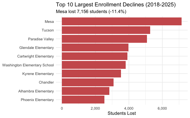
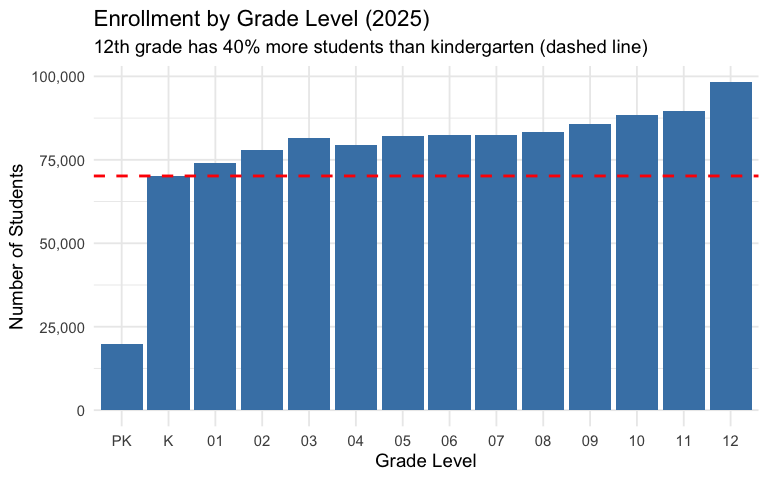
5. Arizona has 40% more seniors than kindergartners
There are 98,216 12th graders but only 70,164 kindergartners - a 40% difference. This “inverted pyramid” could signal declining birth rates or families with young children leaving public schools.
grade_order <- c("PK", "K", "01", "02", "03", "04", "05",
                 "06", "07", "08", "09", "10", "11", "12")

grades <- enr |>
  filter(is_district,
         subgroup == "total_enrollment", grade_level %in% grade_order,
         end_year == 2025) |>
  group_by(grade_level) |>
  summarize(n_students = sum(n_students, na.rm = TRUE), .groups = "drop") |>
  mutate(grade_level = factor(grade_level, levels = grade_order))
stopifnot(nrow(grades) > 0)

grades |>
  arrange(grade_level)
#> # A tibble: 14 × 2
#>    grade_level n_students
#>    <fct>            <dbl>
#>  1 PK               19815
#>  2 K                70164
#>  3 01               73928
#>  4 02               77811
#>  5 03               81507
#>  6 04               79398
#>  7 05               82241
#>  8 06               82458
#>  9 07               82350
#> 10 08               83408
#> 11 09               85720
#> 12 10               88332
#> 13 11               89504
#> 14 12               98216
stopifnot(nrow(grades) > 0)
grades |>
  ggplot(aes(x = grade_level, y = n_students)) +
  geom_col(fill = "#4682B4") +
  geom_hline(yintercept = grades$n_students[grades$grade_level == "K"],
             linetype = "dashed", color = "red", linewidth = 1) +
  scale_y_continuous(labels = scales::comma) +
  labs(
    title = "Enrollment by Grade Level (2025)",
    subtitle = "12th grade has 40% more students than kindergarten (dashed line)",
    x = "Grade Level",
    y = "Number of Students"
  )
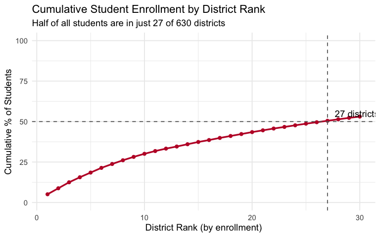
6. Top 27 districts educate half of Arizona’s students
Student enrollment is heavily concentrated: just 27 of Arizona’s 630 districts educate 50% of all students. The top 10 districts alone serve 30% of students.
concentration <- enr |>
  filter(is_district,
         subgroup == "total_enrollment", grade_level == "TOTAL",
         end_year == 2025) |>
  arrange(desc(n_students)) |>
  mutate(
    cum_students = cumsum(n_students),
    cum_pct = round(cum_students / sum(n_students) * 100, 1),
    rank = row_number()
  )
stopifnot(nrow(concentration) > 0)

total_students <- sum(concentration$n_students)
n_districts <- nrow(concentration)

concentration |>
  select(rank, district_name, n_students, cum_pct) |>
  head(15)
#>    rank                         district_name n_students cum_pct
#> 1     1                 Mesa Unified District      55600     5.1
#> 2     2         Chandler Unified District #80      41349     8.8
#> 3     3               Tucson Unified District      40209    12.5
#> 4     4        Peoria Unified School District      34373    15.6
#> 5     5          Deer Valley Unified District      32221    18.5
#> 6     6              Gilbert Unified District      31508    21.4
#> 7     7      Paradise Valley Unified District      26164    23.8
#> 8     8    Phoenix Union High School District      25760    26.1
#> 9     9               Dysart Unified District      23033    28.2
#> 10   10           Scottsdale Unified District      20645    30.1
#> 11   11 Washington Elementary School District      18765    31.8
#> 12   12   Glendale Union High School District      16061    33.3
#> 13   13     American Leadership Academy, Inc.      15266    34.6
#> 14   14          Queen Creek Unified District      15034    36.0
#> 15   15                 Vail Unified District      14941    37.4
conc_top30 <- concentration |>
  filter(rank <= 30)
stopifnot(nrow(conc_top30) > 0)
conc_top30 |>
  ggplot(aes(x = rank, y = cum_pct)) +
  geom_line(color = "#BF0A30", linewidth = 1.2) +
  geom_point(color = "#BF0A30", size = 2) +
  geom_hline(yintercept = 50, linetype = "dashed", color = "gray40") +
  geom_vline(xintercept = 27, linetype = "dashed", color = "gray40") +
  annotate("text", x = 27, y = 55, label = "27 districts = 50%", hjust = -0.1) +
  scale_y_continuous(limits = c(0, 100)) +
  labs(
    title = "Cumulative Student Enrollment by District Rank",
    subtitle = "Half of all students are in just 27 of 630 districts",
    x = "District Rank (by enrollment)",
    y = "Cumulative % of Students"
  )
7. Charters serve nearly 1 in 4 Arizona students
Charter schools and other non-traditional districts now serve 25% of Arizona’s students (270,000 students across 437 districts). Traditional districts (unified, union, elementary) serve the remaining 75%.
charter_data <- enr |>
  filter(is_district,
         subgroup == "total_enrollment", grade_level == "TOTAL",
         end_year == 2025) |>
  mutate(district_type = case_when(
    grepl("Unified|Union|Elementary District|High School District", district_name) ~ "Traditional",
    TRUE ~ "Charter/Other"
  )) |>
  group_by(district_type) |>
  summarize(
    n_districts = n(),
    total_students = sum(n_students, na.rm = TRUE),
    avg_size = round(mean(n_students), 0),
    .groups = "drop"
  ) |>
  mutate(pct = round(total_students / sum(total_students) * 100, 1))
stopifnot(nrow(charter_data) > 0)

charter_data
#> # A tibble: 2 × 5
#>   district_type n_districts total_students avg_size   pct
#>   <chr>               <int>          <dbl>    <dbl> <dbl>
#> 1 Charter/Other         437         270122      618  24.6
#> 2 Traditional           193         829407     4297  75.4
stopifnot(nrow(charter_data) > 0)
charter_data |>
  ggplot(aes(x = district_type, y = total_students, fill = district_type)) +
  geom_col(width = 0.6) +
  geom_text(aes(label = paste0(scales::comma(total_students), "\n(", pct, "%)")),
            vjust = -0.3, size = 4) +
  scale_fill_manual(values = c("Charter/Other" = "#FF8C00", "Traditional" = "#4682B4")) +
  scale_y_continuous(labels = scales::comma, limits = c(0, 1000000)) +
  labs(
    title = "Enrollment by District Type (2025)",
    subtitle = "Charters serve nearly 1 in 4 Arizona students",
    x = NULL,
    y = "Total Students"
  ) +
  theme(legend.position = "none")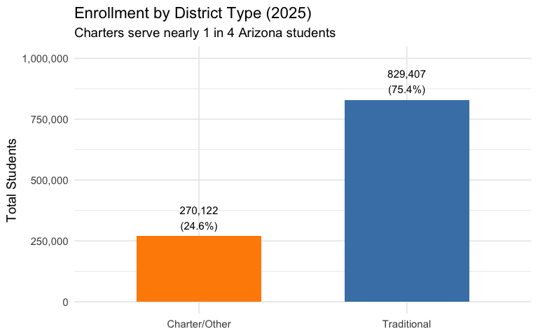
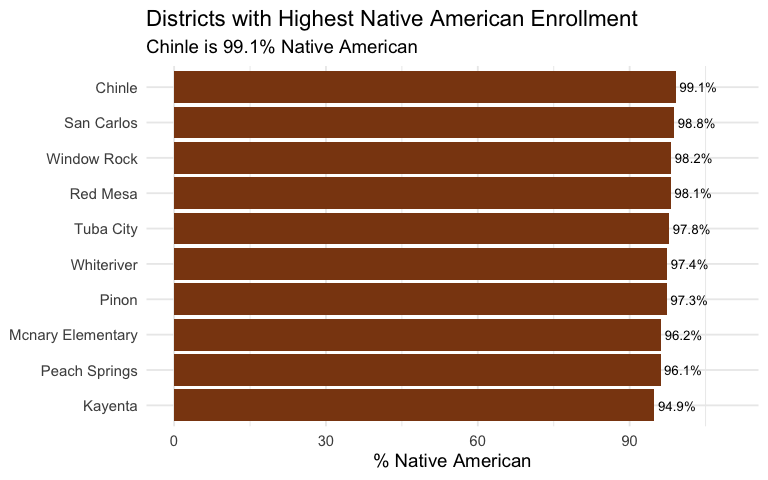
8. Chinle is 99% Native American
Arizona has several districts with almost entirely Native American enrollment, reflecting the state’s 22 federally recognized tribes. Chinle Unified is 99.1% Native American, followed by San Carlos (98.8%) and Window Rock (98.2%).
native_am <- enr |>
  filter(is_district, grade_level == "TOTAL",
         subgroup %in% c("native_american", "total_enrollment"),
         end_year == 2025) |>
  group_by(district_name, subgroup) |>
  summarize(n_students = sum(n_students, na.rm = TRUE), .groups = "drop") |>
  pivot_wider(names_from = subgroup, values_from = n_students) |>
  filter(!is.na(native_american), total_enrollment >= 100) |>
  mutate(pct_native = round(native_american / total_enrollment * 100, 1)) |>
  arrange(desc(pct_native))
stopifnot(nrow(native_am) > 0)

native_am |>
  select(district_name, total_enrollment, native_american, pct_native) |>
  head(10)
#> # A tibble: 10 × 4
#>    district_name                     total_enrollment native_american pct_native
#>    <chr>                                        <dbl>           <dbl>      <dbl>
#>  1 Chinle Unified District                       2908            2882       99.1
#>  2 San Carlos Unified District                   1433            1416       98.8
#>  3 Window Rock Unified District                  1701            1671       98.2
#>  4 Red Mesa Unified District                      427             419       98.1
#>  5 Tuba City Unified School Distric…             1378            1348       97.8
#>  6 Whiteriver Unified District                   2228            2169       97.4
#>  7 Pinon Unified District                        1017             990       97.3
#>  8 Mcnary Elementary District                     183             176       96.2
#>  9 Peach Springs Unified District                 179             172       96.1
#> 10 Kayenta Unified School District …             1540            1461       94.9
native_top10 <- native_am |>
  head(10) |>
  mutate(district_name = gsub(" District.*$| Unified.*$", "", district_name))
stopifnot(nrow(native_top10) > 0)
native_top10 |>
  ggplot(aes(x = reorder(district_name, pct_native), y = pct_native)) +
  geom_col(fill = "#8B4513") +
  geom_text(aes(label = paste0(pct_native, "%")), hjust = -0.1, size = 3.5) +
  coord_flip() +
  scale_y_continuous(limits = c(0, 110)) +
  labs(
    title = "Districts with Highest Native American Enrollment",
    subtitle = "Chinle is 99.1% Native American",
    x = NULL,
    y = "% Native American"
  )
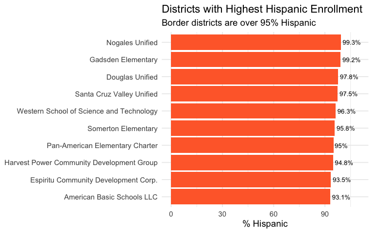
9. Border districts are over 95% Hispanic
Arizona’s border districts have near-complete Hispanic enrollment. Nogales Unified (99.3%), Gadsden Elementary (99.2%), and Douglas Unified (97.8%) serve predominantly Hispanic communities near the Mexico border.
hispanic_maj <- enr |>
  filter(is_district, grade_level == "TOTAL",
         subgroup %in% c("hispanic", "total_enrollment"),
         end_year == 2025) |>
  group_by(district_name, subgroup) |>
  summarize(n_students = sum(n_students, na.rm = TRUE), .groups = "drop") |>
  pivot_wider(names_from = subgroup, values_from = n_students) |>
  filter(!is.na(hispanic), total_enrollment >= 500) |>
  mutate(pct_hispanic = round(hispanic / total_enrollment * 100, 1)) |>
  arrange(desc(pct_hispanic))
stopifnot(nrow(hispanic_maj) > 0)

hispanic_maj |>
  select(district_name, total_enrollment, hispanic, pct_hispanic) |>
  head(10)
#> # A tibble: 10 × 4
#>    district_name                          total_enrollment hispanic pct_hispanic
#>    <chr>                                             <dbl>    <dbl>        <dbl>
#>  1 Nogales Unified District                           5690     5651         99.3
#>  2 Gadsden Elementary District                        5181     5141         99.2
#>  3 Douglas Unified District                           3601     3521         97.8
#>  4 Santa Cruz Valley Unified District                 3606     3516         97.5
#>  5 Western School of Science and Technol…              515      496         96.3
#>  6 Somerton Elementary District                       2967     2843         95.8
#>  7 Pan-American Elementary Charter                    1221     1160         95
#>  8 Harvest Power Community Development G…             1642     1556         94.8
#>  9 Espiritu Community Development Corp.                697      652         93.5
#> 10 American Basic Schools LLC                          634      590         93.1
hispanic_top10 <- hispanic_maj |>
  head(10) |>
  mutate(district_name = gsub(" District.*$|, Inc\\.$", "", district_name))
stopifnot(nrow(hispanic_top10) > 0)
hispanic_top10 |>
  ggplot(aes(x = reorder(district_name, pct_hispanic), y = pct_hispanic)) +
  geom_col(fill = "#FF6B35") +
  geom_text(aes(label = paste0(pct_hispanic, "%")), hjust = -0.1, size = 3.5) +
  coord_flip() +
  scale_y_continuous(limits = c(0, 110)) +
  labs(
    title = "Districts with Highest Hispanic Enrollment",
    subtitle = "Border districts are over 95% Hispanic",
    x = NULL,
    y = "% Hispanic"
  )
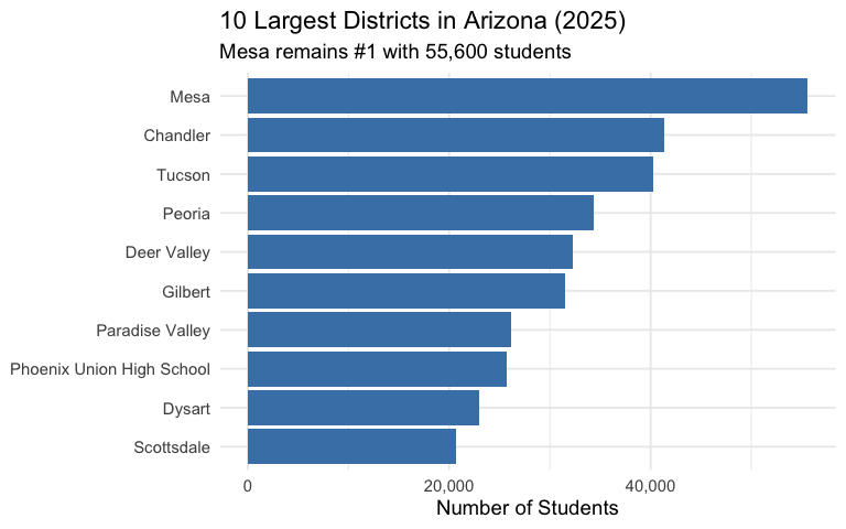
10. Mesa Unified is still Arizona’s largest district
Despite losing 7,156 students, Mesa Unified remains Arizona’s largest district with 55,600 students. Chandler (41,349), Tucson (40,209), and Peoria (34,373) round out the top four.
largest <- enr |>
  filter(is_district,
         subgroup == "total_enrollment", grade_level == "TOTAL",
         end_year == 2025) |>
  select(district_name, n_students) |>
  arrange(desc(n_students))
stopifnot(nrow(largest) > 0)
largest |> head(15)
#>                            district_name n_students
#> 1                  Mesa Unified District      55600
#> 2          Chandler Unified District #80      41349
#> 3                Tucson Unified District      40209
#> 4         Peoria Unified School District      34373
#> 5           Deer Valley Unified District      32221
#> 6               Gilbert Unified District      31508
#> 7       Paradise Valley Unified District      26164
#> 8     Phoenix Union High School District      25760
#> 9                Dysart Unified District      23033
#> 10           Scottsdale Unified District      20645
#> 11 Washington Elementary School District      18765
#> 12   Glendale Union High School District      16061
#> 13     American Leadership Academy, Inc.      15266
#> 14          Queen Creek Unified District      15034
#> 15                 Vail Unified District      14941
largest_top10 <- enr |>
  filter(is_district,
         subgroup == "total_enrollment", grade_level == "TOTAL",
         end_year == 2025) |>
  arrange(desc(n_students)) |>
  head(10) |>
  mutate(district_name = gsub(" District.*$| Unified.*$", "", district_name))
stopifnot(nrow(largest_top10) > 0)
largest_top10 |>
  ggplot(aes(x = reorder(district_name, n_students), y = n_students)) +
  geom_col(fill = "#4682B4") +
  coord_flip() +
  scale_y_continuous(labels = scales::comma) +
  labs(
    title = "10 Largest Districts in Arizona (2025)",
    subtitle = "Mesa remains #1 with 55,600 students",
    x = NULL,
    y = "Number of Students"
  )
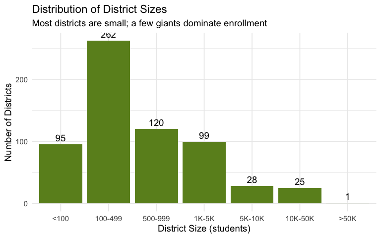
11. Arizona has 630 districts serving 1.1 million students
Arizona’s school system includes 630 separate districts - from Mesa’s 55,600 students down to tiny rural districts with just 11 students. The average district has 1,745 students, but the median is just 414.
district_stats <- enr |>
  filter(is_district,
         subgroup == "total_enrollment", grade_level == "TOTAL",
         end_year == 2025) |>
  summarize(
    n_districts = n(),
    total_students = sum(n_students),
    mean_size = round(mean(n_students), 0),
    median_size = median(n_students),
    min_size = min(n_students),
    max_size = max(n_students)
  )
stopifnot(nrow(district_stats) > 0)

district_stats
#>   n_districts total_students mean_size median_size min_size max_size
#> 1         630        1099529      1745         414       11    55600
size_dist <- enr |>
  filter(is_district,
         subgroup == "total_enrollment", grade_level == "TOTAL",
         end_year == 2025) |>
  mutate(size_bucket = cut(n_students,
                           breaks = c(0, 100, 500, 1000, 5000, 10000, 50000, Inf),
                           labels = c("<100", "100-499", "500-999", "1K-5K",
                                      "5K-10K", "10K-50K", ">50K"))) |>
  count(size_bucket)
stopifnot(nrow(size_dist) > 0)
size_dist |>
  ggplot(aes(x = size_bucket, y = n)) +
  geom_col(fill = "#6B8E23") +
  geom_text(aes(label = n), vjust = -0.5) +
  labs(
    title = "Distribution of District Sizes",
    subtitle = "Most districts are small; a few giants dominate enrollment",
    x = "District Size (students)",
    y = "Number of Districts"
  )
12. Boys outnumber girls 51% to 49%
Male students slightly outnumber female students in Arizona schools: 559,758 boys (50.9%) vs 539,574 girls (49.1%). This 2-point gap is consistent with national patterns.
gender <- enr |>
  filter(is_district, grade_level == "TOTAL",
         subgroup %in% c("male", "female"),
         end_year == 2025) |>
  group_by(subgroup) |>
  summarize(n_students = sum(n_students, na.rm = TRUE), .groups = "drop") |>
  mutate(pct = round(n_students / sum(n_students) * 100, 1))
stopifnot(nrow(gender) > 0)

gender
#> # A tibble: 2 × 3
#>   subgroup n_students   pct
#>   <chr>         <dbl> <dbl>
#> 1 female       539574  49.1
#> 2 male         559758  50.9
stopifnot(nrow(gender) > 0)
gender |>
  ggplot(aes(x = subgroup, y = n_students, fill = subgroup)) +
  geom_col(width = 0.6) +
  geom_text(aes(label = paste0(scales::comma(n_students), "\n(", pct, "%)")),
            vjust = -0.3, size = 4) +
  scale_fill_manual(values = c("female" = "#CC79A7", "male" = "#0072B2")) +
  scale_y_continuous(labels = scales::comma, limits = c(0, 650000)) +
  labs(
    title = "Enrollment by Gender (2025)",
    subtitle = "Boys outnumber girls 51% to 49%",
    x = NULL,
    y = "Number of Students"
  ) +
  theme(legend.position = "none")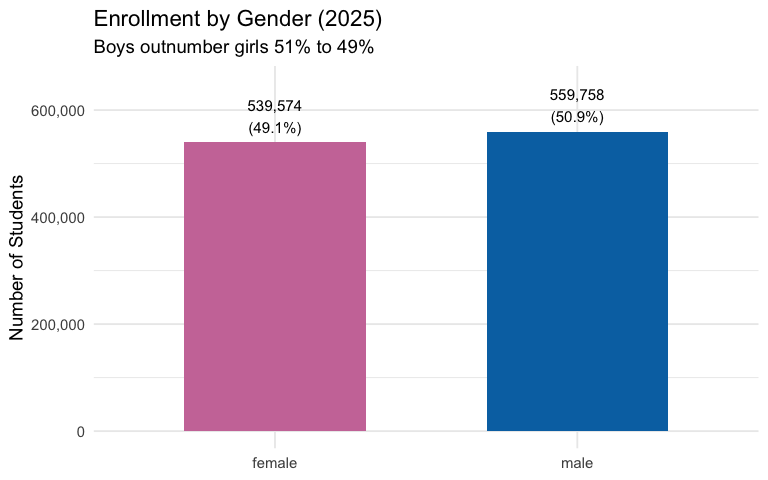
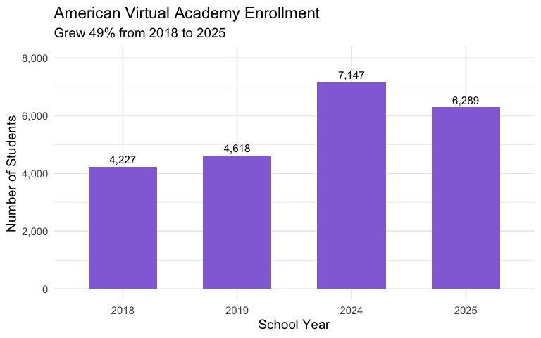
13. Virtual schools serve 6,000+ students
American Virtual Academy is Arizona’s largest virtual school with 6,289 students in 2025. This represents 49% growth from 4,227 students in 2018, reflecting the post-pandemic persistence of online learning.
virtual_schools <- enr |>
  filter(is_district, subgroup == "total_enrollment", grade_level == "TOTAL",
         grepl("Virtual|Online|Digital", district_name, ignore.case = TRUE)) |>
  select(end_year, district_name, n_students) |>
  arrange(end_year, desc(n_students))
stopifnot(nrow(virtual_schools) > 0)
virtual_schools
#>    end_year                   district_name n_students
#> 1      2018        American Virtual Academy       4227
#> 2      2018 ASU Preparatory Academy Digital         38
#> 3      2019        American Virtual Academy       4618
#> 4      2019 ASU Preparatory Academy Digital        276
#> 5      2024        American Virtual Academy       7147
#> 6      2024 ASU Preparatory Academy Digital       3575
#> 7      2024     Premier Prep Online Academy        130
#> 8      2024        Online School of Arizona         41
#> 9      2025        American Virtual Academy       6289
#> 10     2025 ASU Preparatory Academy Digital       3845
#> 11     2025     Premier Prep Online Academy        216
#> 12     2025        Online School of Arizona         45
virtual <- enr |>
  filter(is_district, subgroup == "total_enrollment", grade_level == "TOTAL",
         district_name == "American Virtual Academy")
stopifnot(nrow(virtual) > 0)

virtual |>
  ggplot(aes(x = factor(end_year), y = n_students)) +
  geom_col(fill = "#9370DB", width = 0.6) +
  geom_text(aes(label = scales::comma(n_students)), vjust = -0.5, size = 4) +
  scale_y_continuous(labels = scales::comma, limits = c(0, 8000)) +
  labs(
    title = "American Virtual Academy Enrollment",
    subtitle = "Grew 49% from 2018 to 2025",
    x = "School Year",
    y = "Number of Students"
  )
14. Elementary grades are shrinking faster than high school
Elementary enrollment (K-5) totals 465,049 students while high school (9-12) has 361,772. But when you look at individual grades, high school grades average 90,443 students while elementary grades average only 77,508 - a 17% difference suggesting demographic shift.
grade_groups <- enr |>
  filter(is_district,
         subgroup == "total_enrollment", grade_level %in% grade_order,
         end_year == 2025) |>
  group_by(grade_level) |>
  summarize(n_students = sum(n_students, na.rm = TRUE), .groups = "drop") |>
  mutate(level = case_when(
    grade_level %in% c("K", "01", "02", "03", "04", "05") ~ "Elementary (K-5)",
    grade_level %in% c("06", "07", "08") ~ "Middle (6-8)",
    grade_level %in% c("09", "10", "11", "12") ~ "High School (9-12)",
    TRUE ~ "Other"
  )) |>
  group_by(level) |>
  summarize(
    total_students = sum(n_students),
    n_grades = n(),
    avg_per_grade = round(sum(n_students) / n()),
    .groups = "drop"
  )
stopifnot(nrow(grade_groups) > 0)

grade_groups
#> # A tibble: 4 × 4
#>   level              total_students n_grades avg_per_grade
#>   <chr>                       <dbl>    <int>         <dbl>
#> 1 Elementary (K-5)           465049        6         77508
#> 2 High School (9-12)         361772        4         90443
#> 3 Middle (6-8)               248216        3         82739
#> 4 Other                       19815        1         19815
grade_levels_chart <- grade_groups |>
  filter(level != "Other")
stopifnot(nrow(grade_levels_chart) > 0)
grade_levels_chart |>
  ggplot(aes(x = level, y = avg_per_grade, fill = level)) +
  geom_col(width = 0.6) +
  geom_text(aes(label = scales::comma(avg_per_grade)), vjust = -0.5, size = 4) +
  scale_fill_brewer(palette = "Set1") +
  scale_y_continuous(labels = scales::comma, limits = c(0, 100000)) +
  labs(
    title = "Average Enrollment Per Grade by School Level",
    subtitle = "High school grades average 17% more students than elementary",
    x = NULL,
    y = "Average Students Per Grade"
  ) +
  theme(legend.position = "none")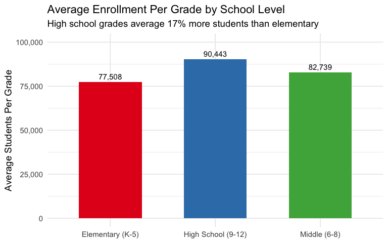
15. 108 districts are Hispanic-majority
Of Arizona’s 630 districts, 108 have majority Hispanic enrollment (at least 500 students and >50% Hispanic). These districts serve 413,175 students total - about 38% of all students statewide.
hispanic_count <- hispanic_maj |>
  filter(pct_hispanic >= 50) |>
  summarize(
    n_districts = n(),
    total_students = sum(total_enrollment),
    pct_of_state = round(sum(total_enrollment) / sum(concentration$n_students) * 100, 1)
  )
stopifnot(nrow(hispanic_count) > 0)

hispanic_count
#> # A tibble: 1 × 3
#>   n_districts total_students pct_of_state
#>         <int>          <dbl>        <dbl>
#> 1         108         413175         37.6
hisp_maj_chart <- hispanic_maj |>
  mutate(majority = ifelse(pct_hispanic >= 50, "Hispanic Majority", "Not Hispanic Majority")) |>
  group_by(majority) |>
  summarize(n_districts = n(), total_students = sum(total_enrollment), .groups = "drop")
stopifnot(nrow(hisp_maj_chart) > 0)
hisp_maj_chart |>
  ggplot(aes(x = majority, y = n_districts, fill = majority)) +
  geom_col(width = 0.6) +
  geom_text(aes(label = paste0(n_districts, " districts\n",
                               scales::comma(total_students), " students")),
            vjust = -0.3, size = 3.5) +
  scale_fill_manual(values = c("Hispanic Majority" = "#FF6B35",
                               "Not Hispanic Majority" = "#4682B4")) +
  scale_y_continuous(limits = c(0, 400)) +
  labs(
    title = "Hispanic-Majority Districts in Arizona",
    subtitle = "108 districts (17%) are majority Hispanic",
    x = NULL,
    y = "Number of Districts"
  ) +
  theme(legend.position = "none")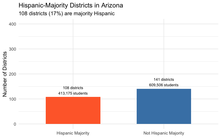
Data Notes
Source: Arizona Department of Education October 1 Enrollment Reports URL: https://www.azed.gov/accountability-research Available years: 2018, 2019, 2024, 2025, 2026 Missing years: 2020-2023 (Cloudflare protection blocks automated downloads)
Important caveats: - Small counts may be suppressed
in the source data (marked with *) - Virtual and charter
schools are counted separately from traditional districts
What’s included: - State, district, and school level enrollment - Demographics: Hispanic, White, Black, Asian, Native American, Pacific Islander, Multiracial - Gender: Male, Female - Grade levels: PK through 12
Session Info
sessionInfo()
#> R version 4.5.2 (2025-10-31)
#> Platform: x86_64-pc-linux-gnu
#> Running under: Ubuntu 24.04.3 LTS
#>
#> Matrix products: default
#> BLAS:   /usr/lib/x86_64-linux-gnu/openblas-pthread/libblas.so.3
#> LAPACK: /usr/lib/x86_64-linux-gnu/openblas-pthread/libopenblasp-r0.3.26.so;  LAPACK version 3.12.0
#>
#> locale:
#>  [1] LC_CTYPE=C.UTF-8       LC_NUMERIC=C           LC_TIME=C.UTF-8
#>  [4] LC_COLLATE=C.UTF-8     LC_MONETARY=C.UTF-8    LC_MESSAGES=C.UTF-8
#>  [7] LC_PAPER=C.UTF-8       LC_NAME=C              LC_ADDRESS=C
#> [10] LC_TELEPHONE=C         LC_MEASUREMENT=C.UTF-8 LC_IDENTIFICATION=C
#>
#> time zone: UTC
#> tzcode source: system (glibc)
#>
#> attached base packages:
#> [1] stats     graphics  grDevices utils     datasets  methods   base
#>
#> other attached packages:
#> [1] ggplot2_4.0.2      tidyr_1.3.2        dplyr_1.2.0        azschooldata_0.1.0
#>
#> loaded via a namespace (and not attached):
#>  [1] gtable_0.3.6       jsonlite_2.0.0     compiler_4.5.2     tidyselect_1.2.1
#>  [5] jquerylib_0.1.4    systemfonts_1.3.2  scales_1.4.0       textshaping_1.0.5
#>  [9] readxl_1.4.5       yaml_2.3.12        fastmap_1.2.0      R6_2.6.1
#> [13] labeling_0.4.3     generics_0.1.4     knitr_1.51         tibble_3.3.1
#> [17] desc_1.4.3         bslib_0.10.0       pillar_1.11.1      RColorBrewer_1.1-3
#> [21] rlang_1.1.7        utf8_1.2.6         cachem_1.1.0       xfun_0.56
#> [25] fs_1.6.7           sass_0.4.10        S7_0.2.1           cli_3.6.5
#> [29] withr_3.0.2        pkgdown_2.2.0      magrittr_2.0.4     digest_0.6.39
#> [33] grid_4.5.2         rappdirs_0.3.4     lifecycle_1.0.5    vctrs_0.7.1
#> [37] evaluate_1.0.5     glue_1.8.0         cellranger_1.1.0   farver_2.1.2
#> [41] codetools_0.2-20   ragg_1.5.1         rmarkdown_2.30     purrr_1.2.1
#> [45] tools_4.5.2        pkgconfig_2.0.3    htmltools_0.5.9