15 Insights from Delaware School Enrollment Data
Source:vignettes/enrollment_hooks.Rmd
enrollment_hooks.Rmd
library(deschooldata)
library(dplyr)
library(tidyr)
library(ggplot2)

theme_set(theme_minimal(base_size = 14))
This vignette explores Delaware’s public school enrollment data, surfacing key trends and demographic patterns across 10 years of data (2015-2024).
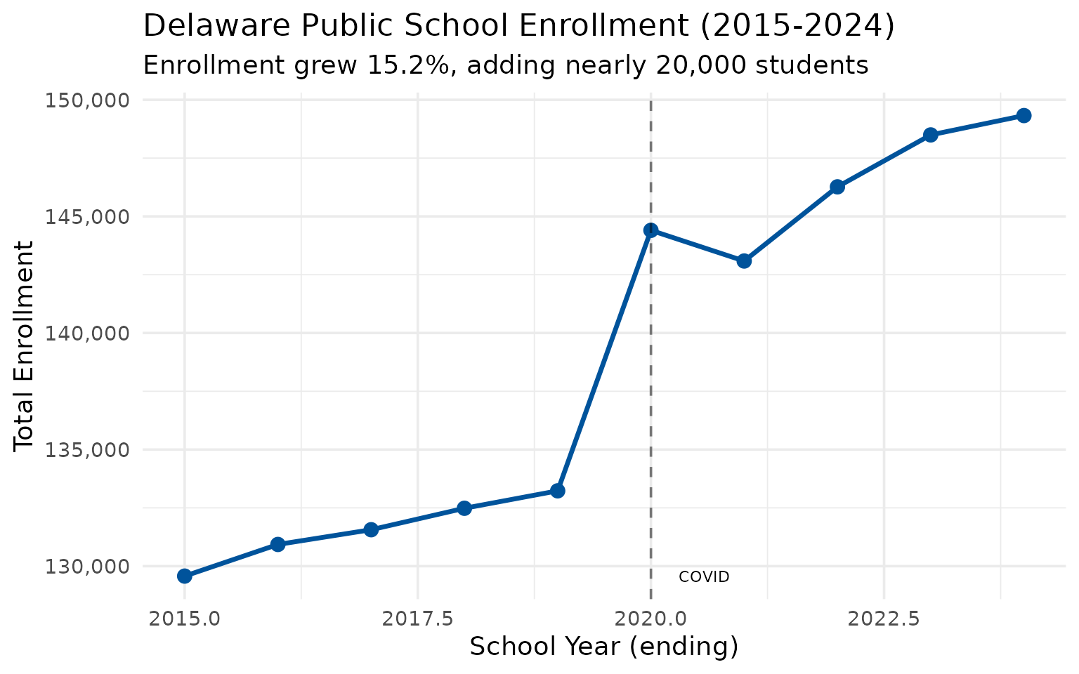
1. Delaware added nearly 20,000 students in a decade
Statewide enrollment grew 15.2% from 129,573 to 149,324 between 2015 and 2024, bucking national enrollment decline trends.
enr <- fetch_enr_multi(2015:2024, use_cache = TRUE)

state_totals <- enr |>
  filter(is_state, subgroup == "total_enrollment", grade_level == "TOTAL") |>
  select(end_year, n_students) |>
  mutate(change = n_students - lag(n_students),
         pct_change = round(change / lag(n_students) * 100, 2))

stopifnot(nrow(state_totals) > 0)
state_totals
#>    end_year n_students change pct_change
#> 1      2015     129573     NA         NA
#> 2      2016     130930   1357       1.05
#> 3      2017     131562    632       0.48
#> 4      2018     132482    920       0.70
#> 5      2019     133230    748       0.56
#> 6      2020     144402  11172       8.39
#> 7      2021     143086  -1316      -0.91
#> 8      2022     146267   3181       2.22
#> 9      2023     148494   2227       1.52
#> 10     2024     149324    830       0.56
ggplot(state_totals, aes(x = end_year, y = n_students)) +
  geom_line(linewidth = 1.2, color = "#00539B") +
  geom_point(size = 3, color = "#00539B") +
  geom_vline(xintercept = 2020, linetype = "dashed", alpha = 0.5) +
  annotate("text", x = 2020.3, y = min(state_totals$n_students),
           label = "COVID", hjust = 0, size = 3) +
  scale_y_continuous(labels = scales::comma) +
  labs(
    title = "Delaware Public School Enrollment (2015-2024)",
    subtitle = "Enrollment grew 15.2%, adding nearly 20,000 students",
    x = "School Year (ending)",
    y = "Total Enrollment"
  )
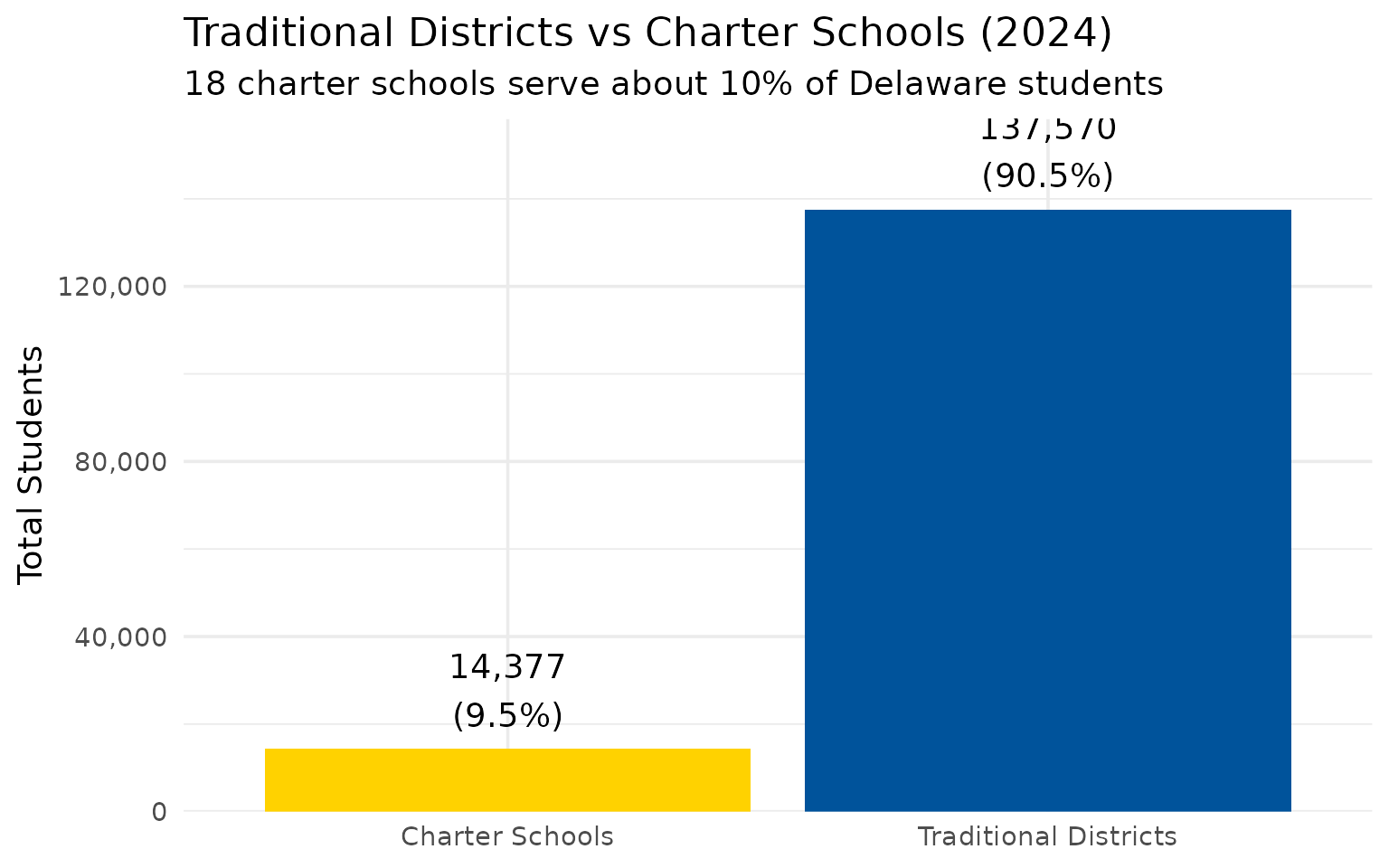
2. Charter schools now serve nearly 10% of Delaware students
Delaware was one of the first states to authorize charter schools (1995). Today 18 charter schools enroll about 14,400 students.
enr_2024 <- fetch_enr(2024, use_cache = TRUE)

charter_summary <- enr_2024 |>
  filter(is_district, subgroup == "total_enrollment", grade_level == "TOTAL") |>
  group_by(is_charter) |>
  summarize(
    n_districts = n(),
    total_students = sum(n_students, na.rm = TRUE),
    .groups = "drop"
  ) |>
  mutate(pct = round(total_students / sum(total_students) * 100, 1))

stopifnot(nrow(charter_summary) == 2)
charter_summary
#> # A tibble: 2 × 4
#>   is_charter n_districts total_students   pct
#>   <lgl>            <int>          <dbl> <dbl>
#> 1 FALSE               22         137570  90.5
#> 2 TRUE                18          14377   9.5
charter_summary |>
  mutate(sector = ifelse(is_charter, "Charter Schools", "Traditional Districts")) |>
  ggplot(aes(x = sector, y = total_students, fill = sector)) +
  geom_col(show.legend = FALSE) +
  geom_text(aes(label = paste0(scales::comma(total_students), "\n(", pct, "%)")),
            vjust = -0.3) +
  scale_y_continuous(labels = scales::comma, expand = expansion(mult = c(0, 0.15))) +
  scale_fill_manual(values = c("Charter Schools" = "#FFD200", "Traditional Districts" = "#00539B")) +
  labs(
    title = "Traditional Districts vs Charter Schools (2024)",
    subtitle = "18 charter schools serve about 10% of Delaware students",
    x = NULL,
    y = "Total Students"
  )
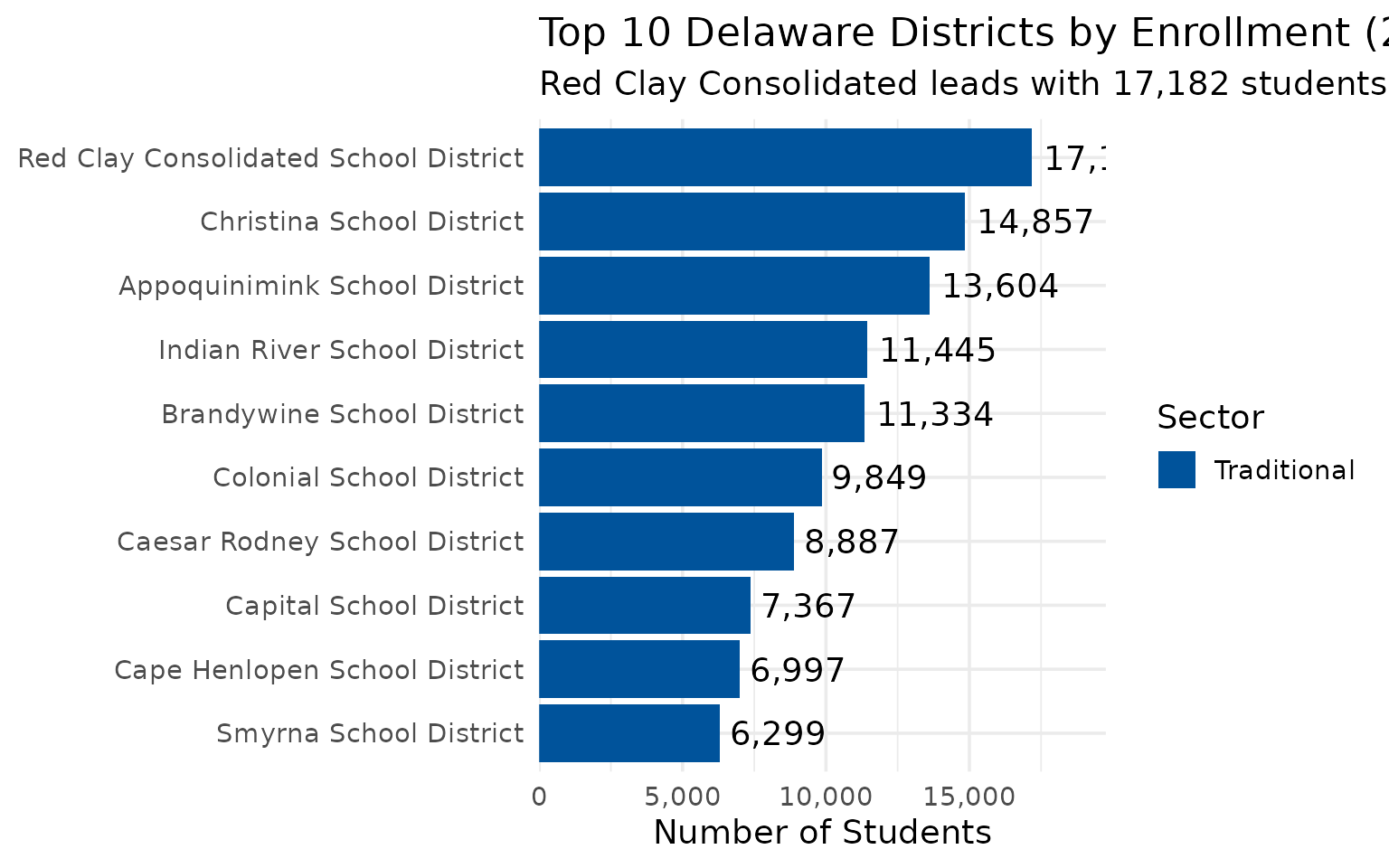
3. Red Clay Consolidated leads Delaware’s 40 districts
With 17,182 students, Red Clay Consolidated is the state’s largest district. The top 10 include both New Castle County giants and a charter school.
top_districts <- enr_2024 |>
  filter(is_district, subgroup == "total_enrollment", grade_level == "TOTAL") |>
  arrange(desc(n_students)) |>
  head(10) |>
  select(district_name, n_students, is_charter)

stopifnot(nrow(top_districts) == 10)
top_districts
#>                            district_name n_students is_charter
#> 1  Red Clay Consolidated School District      17182      FALSE
#> 2              Christina School District      14857      FALSE
#> 3          Appoquinimink School District      13604      FALSE
#> 4           Indian River School District      11445      FALSE
#> 5             Brandywine School District      11334      FALSE
#> 6               Colonial School District       9849      FALSE
#> 7          Caesar Rodney School District       8887      FALSE
#> 8                Capital School District       7367      FALSE
#> 9          Cape Henlopen School District       6997      FALSE
#> 10                Smyrna School District       6299      FALSE
top_districts |>
  mutate(district_name = forcats::fct_reorder(district_name, n_students),
         sector = ifelse(is_charter, "Charter", "Traditional")) |>
  ggplot(aes(x = n_students, y = district_name, fill = sector)) +
  geom_col() +
  geom_text(aes(label = scales::comma(n_students)), hjust = -0.1) +
  scale_x_continuous(labels = scales::comma, expand = expansion(mult = c(0, 0.15))) +
  scale_fill_manual(values = c("Charter" = "#FFD200", "Traditional" = "#00539B")) +
  labs(
    title = "Top 10 Delaware Districts by Enrollment (2024)",
    subtitle = "Red Clay Consolidated leads with 17,182 students",
    x = "Number of Students",
    y = NULL,
    fill = "Sector"
  )
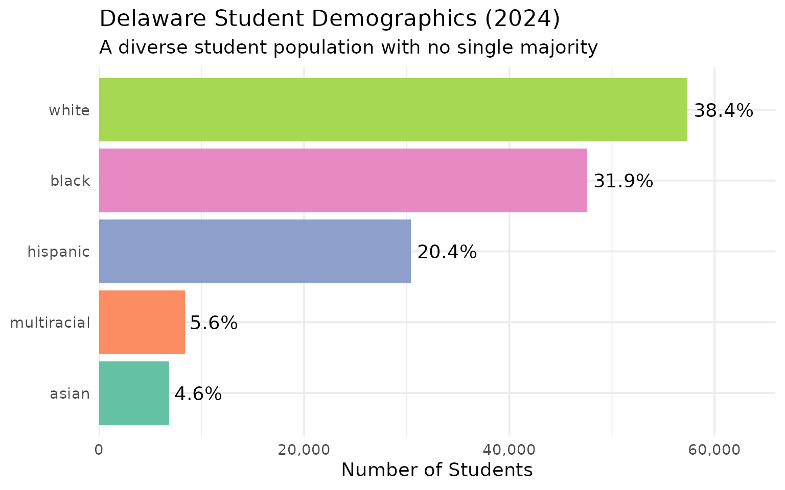
4. Delaware is remarkably diverse
No single racial group holds a majority. White students are the plurality at 38.4%, followed by Black (31.9%) and Hispanic (20.4%).
demographics <- enr_2024 |>
  filter(is_state, grade_level == "TOTAL",
         subgroup %in% c("white", "black", "hispanic", "asian", "multiracial")) |>
  mutate(pct = round(pct * 100, 1)) |>
  select(subgroup, n_students, pct) |>
  arrange(desc(n_students))

stopifnot(nrow(demographics) > 0)
demographics
#>      subgroup n_students  pct
#> 1       white      57336 38.4
#> 2       black      47582 31.9
#> 3    hispanic      30395 20.4
#> 4 multiracial       8389  5.6
#> 5       asian       6865  4.6
demographics |>
  mutate(subgroup = forcats::fct_reorder(subgroup, n_students)) |>
  ggplot(aes(x = n_students, y = subgroup, fill = subgroup)) +
  geom_col(show.legend = FALSE) +
  geom_text(aes(label = paste0(pct, "%")), hjust = -0.1) +
  scale_x_continuous(labels = scales::comma, expand = expansion(mult = c(0, 0.15))) +
  scale_fill_brewer(palette = "Set2") +
  labs(
    title = "Delaware Student Demographics (2024)",
    subtitle = "A diverse student population with no single majority",
    x = "Number of Students",
    y = NULL
  )
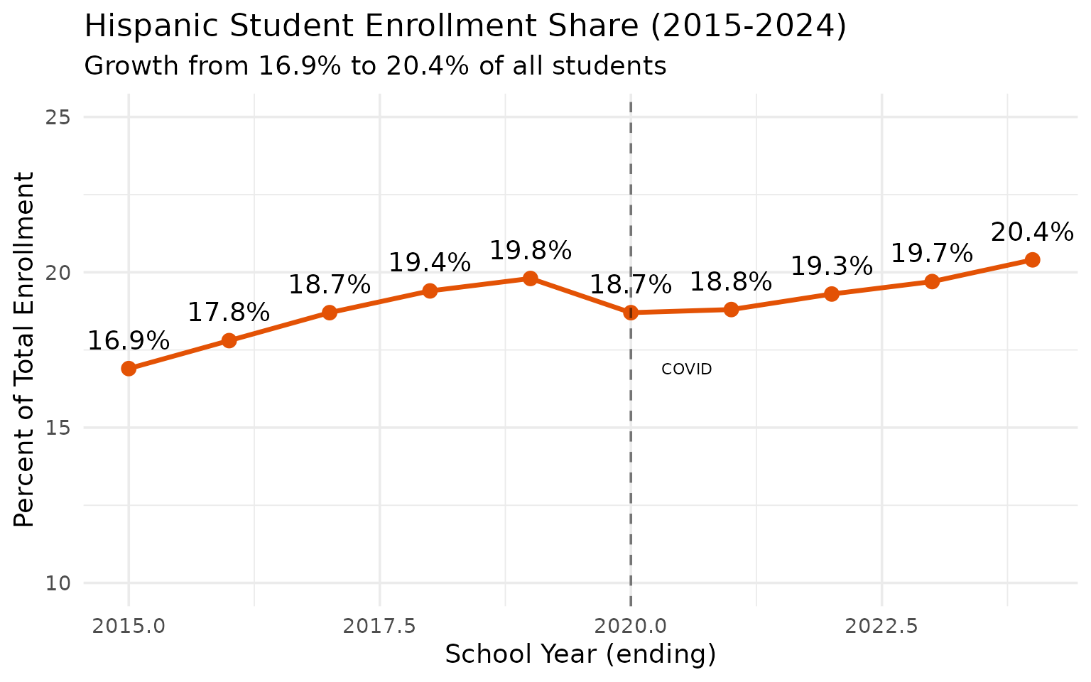
5. Hispanic enrollment grew from 17% to 20% in a decade
Hispanic students went from 21,902 (16.9%) in 2015 to 30,395 (20.4%) in 2024, an increase of nearly 8,500 students.
hispanic_trend <- enr |>
  filter(is_state, subgroup == "hispanic", grade_level == "TOTAL") |>
  mutate(pct = round(pct * 100, 1)) |>
  select(end_year, n_students, pct)

stopifnot(nrow(hispanic_trend) > 0)
hispanic_trend
#>    end_year n_students  pct
#> 1      2015      21902 16.9
#> 2      2016      23269 17.8
#> 3      2017      24604 18.7
#> 4      2018      25714 19.4
#> 5      2019      26313 19.8
#> 6      2020      26947 18.7
#> 7      2021      26882 18.8
#> 8      2022      28299 19.3
#> 9      2023      29245 19.7
#> 10     2024      30395 20.4
ggplot(hispanic_trend, aes(x = end_year, y = pct)) +
  geom_line(linewidth = 1.2, color = "#E35205") +
  geom_point(size = 3, color = "#E35205") +
  geom_text(aes(label = paste0(pct, "%")), vjust = -1) +
  geom_vline(xintercept = 2020, linetype = "dashed", alpha = 0.5) +
  annotate("text", x = 2020.3, y = min(hispanic_trend$pct),
           label = "COVID", hjust = 0, size = 3) +
  scale_y_continuous(limits = c(10, 25)) +
  labs(
    title = "Hispanic Student Enrollment Share (2015-2024)",
    subtitle = "Growth from 16.9% to 20.4% of all students",
    x = "School Year (ending)",
    y = "Percent of Total Enrollment"
  )
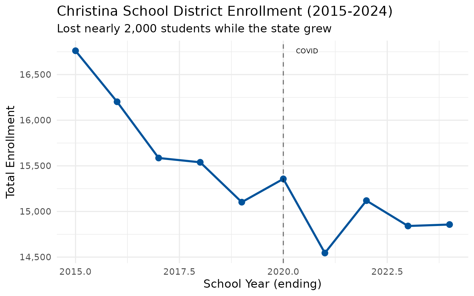
6. Christina School District lost nearly 2,000 students
Christina dropped from 16,761 to 14,857 students between 2015 and 2024, a decline of 11.4% even as the state grew.
christina <- enr |>
  filter(is_district, subgroup == "total_enrollment", grade_level == "TOTAL",
         grepl("Christina", district_name)) |>
  select(end_year, district_name, n_students) |>
  mutate(change = n_students - lag(n_students))

stopifnot(nrow(christina) > 0)
christina
#>    end_year             district_name n_students change
#> 1      2015 Christina School District      16761     NA
#> 2      2016 Christina School District      16202   -559
#> 3      2017 Christina School District      15586   -616
#> 4      2018 Christina School District      15539    -47
#> 5      2019 Christina School District      15102   -437
#> 6      2020 Christina School District      15357    255
#> 7      2021 Christina School District      14545   -812
#> 8      2022 Christina School District      15119    574
#> 9      2023 Christina School District      14841   -278
#> 10     2024 Christina School District      14857     16
ggplot(christina, aes(x = end_year, y = n_students)) +
  geom_line(linewidth = 1.2, color = "#00539B") +
  geom_point(size = 3, color = "#00539B") +
  geom_vline(xintercept = 2020, linetype = "dashed", alpha = 0.5) +
  annotate("text", x = 2020.3, y = max(christina$n_students),
           label = "COVID", hjust = 0, size = 3) +
  scale_y_continuous(labels = scales::comma) +
  labs(
    title = "Christina School District Enrollment (2015-2024)",
    subtitle = "Lost nearly 2,000 students while the state grew",
    x = "School Year (ending)",
    y = "Total Enrollment"
  )
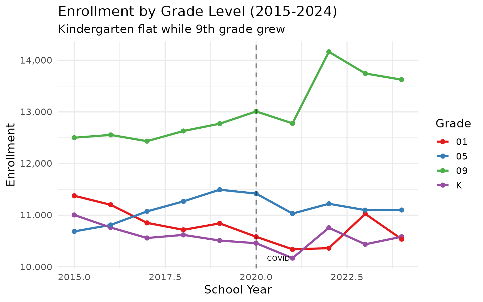
7. Kindergarten enrollment has softened
Delaware’s kindergarten enrollment dropped from 11,004 in 2015 to 10,582 in 2024, even as total enrollment grew. A potential early warning sign.
grade_trends <- enr |>
  filter(is_state, subgroup == "total_enrollment",
         grade_level %in% c("K", "01", "05", "09")) |>
  select(end_year, grade_level, n_students) |>
  pivot_wider(names_from = grade_level, values_from = n_students)

stopifnot(nrow(grade_trends) > 0)
grade_trends
#> # A tibble: 10 × 5
#>    end_year     K  `01`  `05`  `09`
#>       <int> <dbl> <dbl> <dbl> <dbl>
#>  1     2015 11004 11376 10686 12500
#>  2     2016 10761 11201 10810 12554
#>  3     2017 10558 10851 11073 12433
#>  4     2018 10618 10716 11267 12630
#>  5     2019 10509 10841 11493 12771
#>  6     2020 10457 10582 11418 13009
#>  7     2021 10168 10339 11031 12778
#>  8     2022 10756 10361 11221 14164
#>  9     2023 10436 11026 11098 13744
#> 10     2024 10582 10536 11100 13624
kg_data <- enr |>
  filter(is_state, subgroup == "total_enrollment",
         grade_level %in% c("K", "01", "05", "09"))

stopifnot(nrow(kg_data) > 0)

ggplot(kg_data, aes(x = end_year, y = n_students, color = grade_level)) +
  geom_line(linewidth = 1.2) +
  geom_point(size = 2) +
  geom_vline(xintercept = 2020, linetype = "dashed", alpha = 0.5) +
  annotate("text", x = 2020.3, y = min(kg_data$n_students),
           label = "COVID", hjust = 0, size = 3) +
  scale_y_continuous(labels = scales::comma) +
  scale_color_brewer(palette = "Set1") +
  labs(
    title = "Enrollment by Grade Level (2015-2024)",
    subtitle = "Kindergarten flat while 9th grade grew",
    x = "School Year",
    y = "Enrollment",
    color = "Grade"
  )
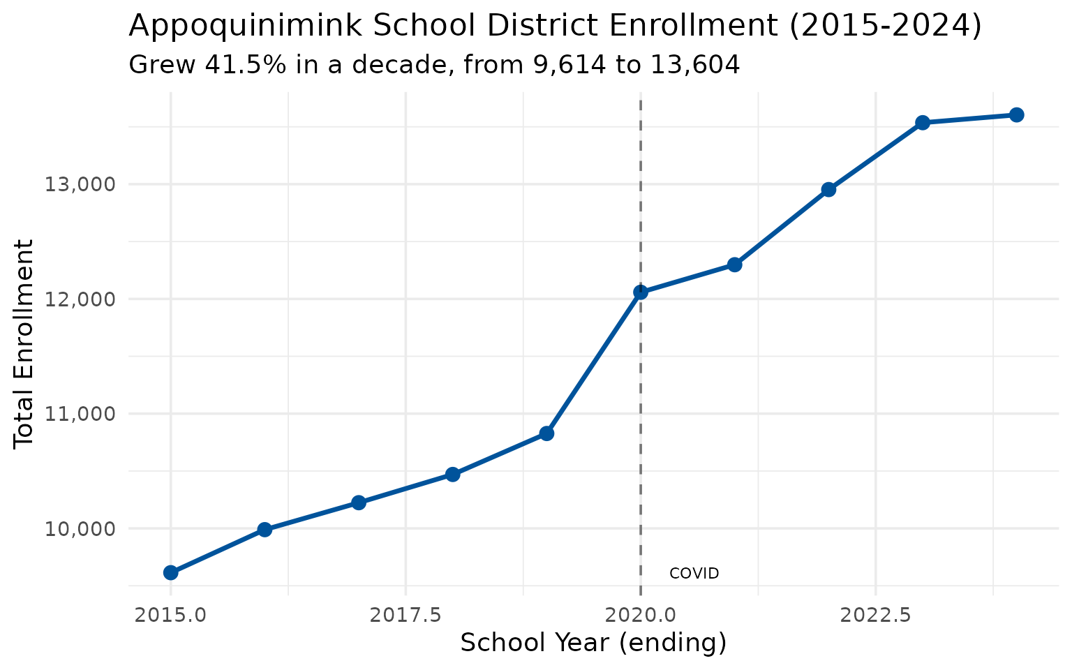
8. Appoquinimink is Delaware’s fastest-growing large district
Appoquinimink grew from 9,614 to 13,604 students (+41.5%), driven by suburban growth south of Wilmington.
appo <- enr |>
  filter(is_district, subgroup == "total_enrollment", grade_level == "TOTAL",
         grepl("Appoquinimink", district_name)) |>
  select(end_year, district_name, n_students) |>
  mutate(change = n_students - lag(n_students))

stopifnot(nrow(appo) > 0)
appo
#>    end_year                 district_name n_students change
#> 1      2015 Appoquinimink School District       9614     NA
#> 2      2016 Appoquinimink School District       9989    375
#> 3      2017 Appoquinimink School District      10224    235
#> 4      2018 Appoquinimink School District      10470    246
#> 5      2019 Appoquinimink School District      10827    357
#> 6      2020 Appoquinimink School District      12058   1231
#> 7      2021 Appoquinimink School District      12298    240
#> 8      2022 Appoquinimink School District      12953    655
#> 9      2023 Appoquinimink School District      13536    583
#> 10     2024 Appoquinimink School District      13604     68
ggplot(appo, aes(x = end_year, y = n_students)) +
  geom_line(linewidth = 1.2, color = "#00539B") +
  geom_point(size = 3, color = "#00539B") +
  geom_vline(xintercept = 2020, linetype = "dashed", alpha = 0.5) +
  annotate("text", x = 2020.3, y = min(appo$n_students),
           label = "COVID", hjust = 0, size = 3) +
  scale_y_continuous(labels = scales::comma) +
  labs(
    title = "Appoquinimink School District Enrollment (2015-2024)",
    subtitle = "Grew 41.5% in a decade, from 9,614 to 13,604",
    x = "School Year (ending)",
    y = "Total Enrollment"
  )
9. Sussex County schools are booming
Southern Delaware’s Sussex County districts have grown faster than the rest of the state, led by Cape Henlopen (+41%) and Indian River (+18%).
sussex_districts <- enr |>
filter(is_district, subgroup == "total_enrollment", grade_level == "TOTAL",
grepl("Sussex|Cape Henlopen|Indian River", district_name)) |>
group_by(district_name) |>
filter(n() > 5) |>
summarize(
earliest = n_students[end_year == min(end_year)],
latest = n_students[end_year == max(end_year)],
pct_change = round((latest / earliest - 1) * 100, 1),
.groups = "drop"
) |>
arrange(desc(pct_change))
stopifnot(nrow(sussex_districts) > 0)
sussex_districts
#> # A tibble: 4 × 4
#> district_name earliest latest pct_change
#> <chr> <dbl> <dbl> <dbl>
#> 1 Sussex Academy 609 1181 93.9
#> 2 Cape Henlopen School District 4960 6997 41.1
#> 3 Indian River School District 9684 11445 18.2
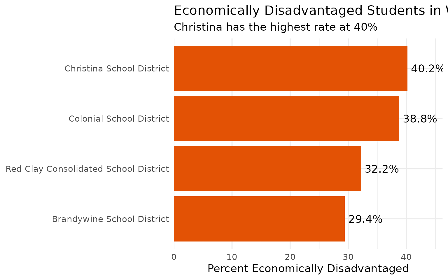
#> 4 Sussex Technical School District 1289 980 -2410. Wilmington-area districts serve more low-income students
The four largest New Castle County districts – Christina, Red Clay, Colonial, and Brandywine – all have substantial economically disadvantaged populations, ranging from 29% to 40%.
wilmington_area <- enr_2024 |>
filter(is_district, grade_level == "TOTAL",
grepl("Brandywine|Red Clay|Christina|Colonial", district_name),
subgroup %in% c("total_enrollment", "econ_disadv")) |>
select(district_name, subgroup, n_students, pct) |>
pivot_wider(names_from = subgroup, values_from = c(n_students, pct))
stopifnot(nrow(wilmington_area) > 0)
wilmington_area
#> # A tibble: 4 × 5
#> district_name n_students_total_enr…¹ n_students_econ_disadv
#> <chr> <dbl> <dbl>
#> 1 Brandywine School District 11334 3330
#> 2 Red Clay Consolidated School Di… 17182 5538
#> 3 Christina School District 14857 5975
#> 4 Colonial School District 9849 3820
#> # ℹ abbreviated name: ¹n_students_total_enrollment
#> # ℹ 2 more variables: pct_total_enrollment <dbl>, pct_econ_disadv <dbl>
wilm_econ <- enr_2024 |>
  filter(is_district, grade_level == "TOTAL",
         grepl("Brandywine|Red Clay|Christina|Colonial", district_name),
         subgroup == "econ_disadv") |>
  mutate(pct_display = round(pct * 100, 1))

stopifnot(nrow(wilm_econ) > 0)

wilm_econ |>
  mutate(district_name = forcats::fct_reorder(district_name, pct_display)) |>
  ggplot(aes(x = pct_display, y = district_name)) +
  geom_col(fill = "#E35205") +
  geom_text(aes(label = paste0(pct_display, "%")), hjust = -0.1) +
  scale_x_continuous(expand = expansion(mult = c(0, 0.15))) +
  labs(
    title = "Economically Disadvantaged Students in Wilmington-Area Districts (2024)",
    subtitle = "Christina has the highest rate at 40%",
    x = "Percent Economically Disadvantaged",
    y = NULL
  )
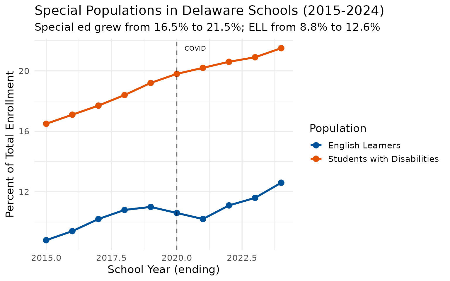
11. One in five Delaware students receives special education
Special education enrollment has grown from 16.5% to 21.5% of all students over the past decade, and English learners grew from 8.8% to 12.6%.
special_pops <- enr |>
  filter(is_state, grade_level == "TOTAL",
         subgroup %in% c("lep", "special_ed")) |>
  select(end_year, subgroup, n_students, pct) |>
  mutate(pct = round(pct * 100, 1))

stopifnot(nrow(special_pops) > 0)
special_pops
#>    end_year   subgroup n_students  pct
#> 1      2015 special_ed      21361 16.5
#> 2      2015        lep      11354  8.8
#> 3      2016 special_ed      22349 17.1
#> 4      2016        lep      12248  9.4
#> 5      2017 special_ed      23351 17.7
#> 6      2017        lep      13451 10.2
#> 7      2018 special_ed      24440 18.4
#> 8      2018        lep      14342 10.8
#> 9      2019 special_ed      25614 19.2
#> 10     2019        lep      14717 11.0
#> 11     2020 special_ed      28621 19.8
#> 12     2020        lep      15295 10.6
#> 13     2021 special_ed      28889 20.2
#> 14     2021        lep      14650 10.2
#> 15     2022 special_ed      30145 20.6
#> 16     2022        lep      16189 11.1
#> 17     2023 special_ed      31071 20.9
#> 18     2023        lep      17171 11.6
#> 19     2024 special_ed      32138 21.5
#> 20     2024        lep      18774 12.6
special_pops |>
  mutate(subgroup = case_when(
    subgroup == "lep" ~ "English Learners",
    subgroup == "special_ed" ~ "Students with Disabilities",
    TRUE ~ subgroup
  )) |>
  ggplot(aes(x = end_year, y = pct, color = subgroup)) +
  geom_line(linewidth = 1.2) +
  geom_point(size = 3) +
  geom_vline(xintercept = 2020, linetype = "dashed", alpha = 0.5) +
  annotate("text", x = 2020.3, y = max(special_pops$pct),
           label = "COVID", hjust = 0, size = 3) +
  scale_color_manual(values = c("English Learners" = "#00539B", "Students with Disabilities" = "#E35205")) +
  labs(
    title = "Special Populations in Delaware Schools (2015-2024)",
    subtitle = "Special ed grew from 16.5% to 21.5%; ELL from 8.8% to 12.6%",
    x = "School Year (ending)",
    y = "Percent of Total Enrollment",
    color = "Population"
  )
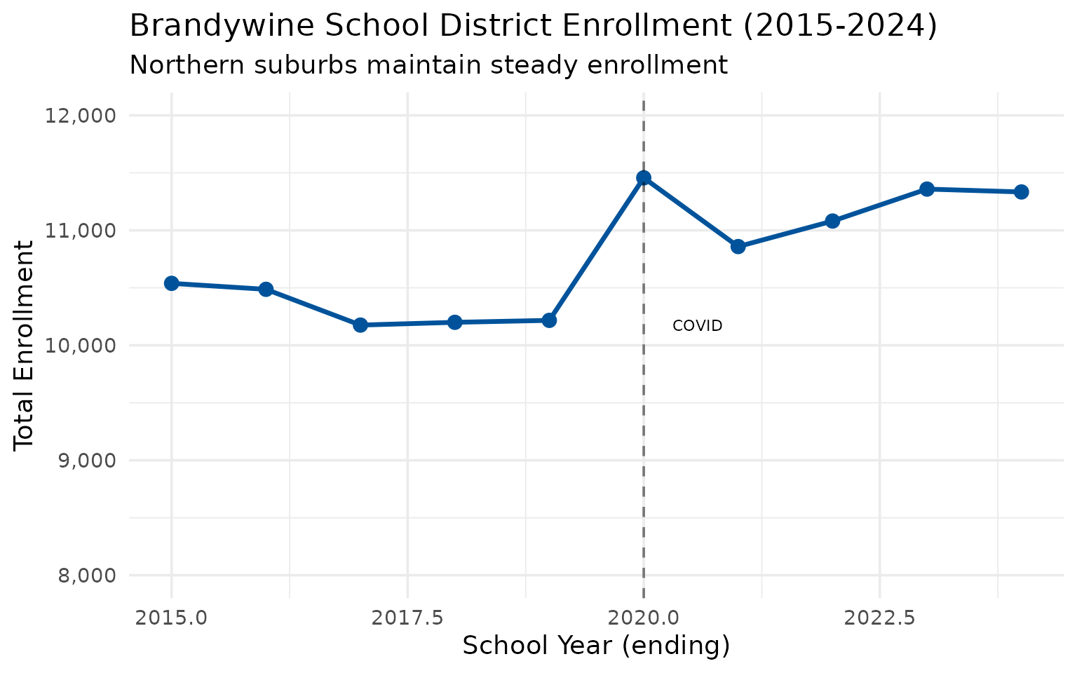
12. Brandywine holds steady while neighbors shrink
Brandywine School District has maintained relatively stable enrollment around 10,200-11,300 while Christina lost nearly 2,000 students.
brandywine <- enr |>
  filter(is_district, subgroup == "total_enrollment", grade_level == "TOTAL",
         grepl("Brandywine", district_name)) |>
  select(end_year, district_name, n_students) |>
  mutate(change = n_students - lag(n_students),
         pct_change = round(change / lag(n_students) * 100, 1))

stopifnot(nrow(brandywine) > 0)
brandywine
#>    end_year              district_name n_students change pct_change
#> 1      2015 Brandywine School District      10539     NA         NA
#> 2      2016 Brandywine School District      10487    -52       -0.5
#> 3      2017 Brandywine School District      10176   -311       -3.0
#> 4      2018 Brandywine School District      10200     24        0.2
#> 5      2019 Brandywine School District      10217     17        0.2
#> 6      2020 Brandywine School District      11457   1240       12.1
#> 7      2021 Brandywine School District      10859   -598       -5.2
#> 8      2022 Brandywine School District      11081    222        2.0
#> 9      2023 Brandywine School District      11359    278        2.5
#> 10     2024 Brandywine School District      11334    -25       -0.2
ggplot(brandywine, aes(x = end_year, y = n_students)) +
  geom_line(linewidth = 1.2, color = "#00539B") +
  geom_point(size = 3, color = "#00539B") +
  geom_vline(xintercept = 2020, linetype = "dashed", alpha = 0.5) +
  annotate("text", x = 2020.3, y = min(brandywine$n_students),
           label = "COVID", hjust = 0, size = 3) +
  scale_y_continuous(labels = scales::comma, limits = c(8000, 12000)) +
  labs(
    title = "Brandywine School District Enrollment (2015-2024)",
    subtitle = "Northern suburbs maintain steady enrollment",
    x = "School Year (ending)",
    y = "Total Enrollment"
  )
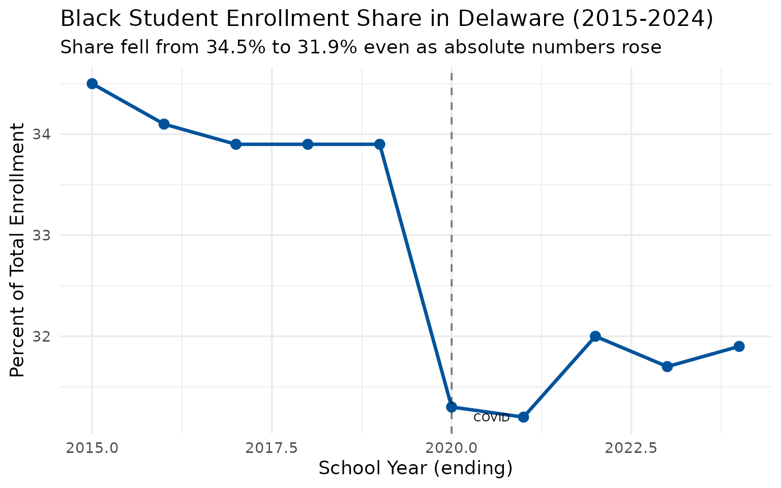
13. Black student share is declining even as numbers rise
Black student enrollment actually grew from 44,700 to 47,582 (+6.4%), but their share of total enrollment fell from 34.5% to 31.9% as Hispanic and other groups grew faster.
black_trend <- enr |>
  filter(is_state, subgroup == "black", grade_level == "TOTAL") |>
  mutate(pct = round(pct * 100, 1)) |>
  select(end_year, n_students, pct)

stopifnot(nrow(black_trend) > 0)
black_trend
#>    end_year n_students  pct
#> 1      2015      44700 34.5
#> 2      2016      44644 34.1
#> 3      2017      44603 33.9
#> 4      2018      44970 33.9
#> 5      2019      45112 33.9
#> 6      2020      45227 31.3
#> 7      2021      44708 31.2
#> 8      2022      46822 32.0
#> 9      2023      47108 31.7
#> 10     2024      47582 31.9
ggplot(black_trend, aes(x = end_year, y = pct)) +
  geom_line(linewidth = 1.2, color = "#00539B") +
  geom_point(size = 3, color = "#00539B") +
  geom_vline(xintercept = 2020, linetype = "dashed", alpha = 0.5) +
  annotate("text", x = 2020.3, y = min(black_trend$pct),
           label = "COVID", hjust = 0, size = 3) +
  labs(
    title = "Black Student Enrollment Share in Delaware (2015-2024)",
    subtitle = "Share fell from 34.5% to 31.9% even as absolute numbers rose",
    x = "School Year (ending)",
    y = "Percent of Total Enrollment"
  )
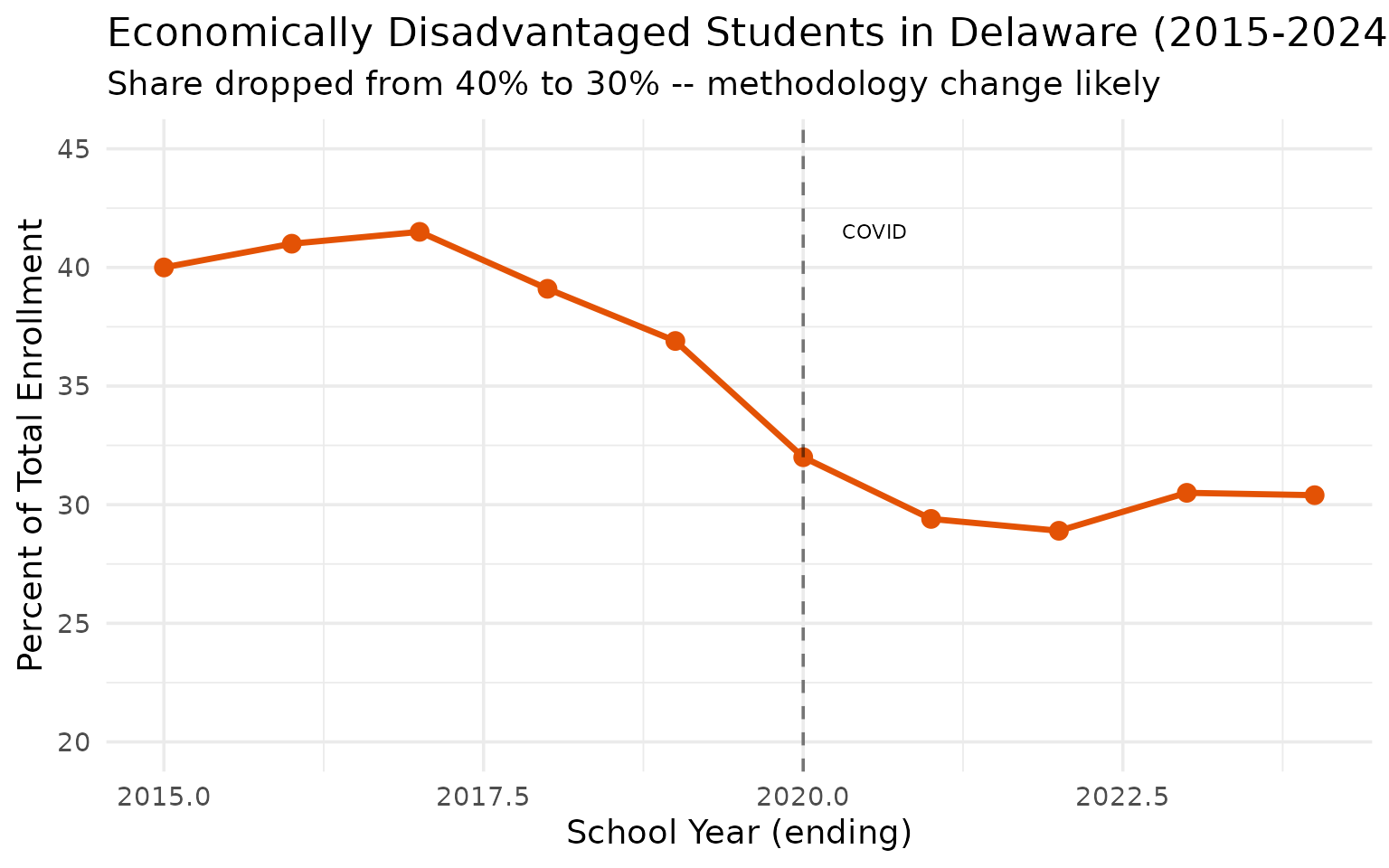
14. Economically disadvantaged share dropped from 40% to 30%
The share of students classified as economically disadvantaged fell from 40.0% in 2015 to 30.4% in 2024. This may reflect changes in reporting methodology rather than actual income gains.
econ_trend <- enr |>
  filter(is_state, grade_level == "TOTAL", subgroup == "econ_disadv") |>
  mutate(pct = round(pct * 100, 1)) |>
  select(end_year, n_students, pct)

stopifnot(nrow(econ_trend) > 0)
econ_trend
#>    end_year n_students  pct
#> 1      2015      51854 40.0
#> 2      2016      53712 41.0
#> 3      2017      54564 41.5
#> 4      2018      51759 39.1
#> 5      2019      49102 36.9
#> 6      2020      46186 32.0
#> 7      2021      42138 29.4
#> 8      2022      42250 28.9
#> 9      2023      45255 30.5
#> 10     2024      45467 30.4
ggplot(econ_trend, aes(x = end_year, y = pct)) +
  geom_line(linewidth = 1.2, color = "#E35205") +
  geom_point(size = 3, color = "#E35205") +
  geom_vline(xintercept = 2020, linetype = "dashed", alpha = 0.5) +
  annotate("text", x = 2020.3, y = max(econ_trend$pct),
           label = "COVID", hjust = 0, size = 3) +
  scale_y_continuous(limits = c(20, 45)) +
  labs(
    title = "Economically Disadvantaged Students in Delaware (2015-2024)",
    subtitle = "Share dropped from 40% to 30% -- methodology change likely",
    x = "School Year (ending)",
    y = "Percent of Total Enrollment"
  )
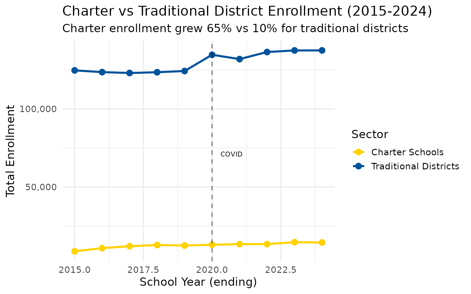
15. Charter enrollment grew 65% while traditional districts grew 10%
Charter schools grew from 8,714 to 14,377 students (65% increase) while traditional district enrollment grew from 124,759 to 137,570 (10%).
charter_trend <- enr |>
  filter(is_district, subgroup == "total_enrollment", grade_level == "TOTAL") |>
  group_by(end_year, is_charter) |>
  summarize(total = sum(n_students, na.rm = TRUE), .groups = "drop") |>
  mutate(sector = ifelse(is_charter, "Charter Schools", "Traditional Districts"))

stopifnot(nrow(charter_trend) > 0)
charter_trend
#> # A tibble: 20 × 4
#>    end_year is_charter  total sector
#>       <int> <lgl>       <dbl> <chr>
#>  1     2015 FALSE      124759 Traditional Districts
#>  2     2015 TRUE         8714 Charter Schools
#>  3     2016 FALSE      123646 Traditional Districts
#>  4     2016 TRUE        10739 Charter Schools
#>  5     2017 FALSE      123075 Traditional Districts
#>  6     2017 TRUE        11982 Charter Schools
#>  7     2018 FALSE      123573 Traditional Districts
#>  8     2018 TRUE        12717 Charter Schools
#>  9     2019 FALSE      124350 Traditional Districts
#> 10     2019 TRUE        12440 Charter Schools
#> 11     2020 FALSE      134768 Traditional Districts
#> 12     2020 TRUE        12904 Charter Schools
#> 13     2021 FALSE      131997 Traditional Districts
#> 14     2021 TRUE        13300 Charter Schools
#> 15     2022 FALSE      136543 Traditional Districts
#> 16     2022 TRUE        13320 Charter Schools
#> 17     2023 FALSE      137542 Traditional Districts
#> 18     2023 TRUE        14552 Charter Schools
#> 19     2024 FALSE      137570 Traditional Districts
#> 20     2024 TRUE        14377 Charter Schools
ggplot(charter_trend, aes(x = end_year, y = total, color = sector)) +
  geom_line(linewidth = 1.2) +
  geom_point(size = 3) +
  geom_vline(xintercept = 2020, linetype = "dashed", alpha = 0.5) +
  annotate("text", x = 2020.3, y = mean(charter_trend$total),
           label = "COVID", hjust = 0, size = 3) +
  scale_y_continuous(labels = scales::comma) +
  scale_color_manual(values = c("Charter Schools" = "#FFD200", "Traditional Districts" = "#00539B")) +
  labs(
    title = "Charter vs Traditional District Enrollment (2015-2024)",
    subtitle = "Charter enrollment grew 65% vs 10% for traditional districts",
    x = "School Year (ending)",
    y = "Total Enrollment",
    color = "Sector"
  )
Summary
Delaware’s school enrollment data reveals: - Strong growth: +15.2%, adding nearly 20,000 students in a decade - Charter pioneer: 18 charter schools now serve nearly 10% of students - Diverse population: No single racial majority – 38% white, 32% Black, 20% Hispanic - Hispanic growth: From 16.9% to 20.4% over a decade - Black share declining: Despite absolute numbers rising, share fell from 34.5% to 31.9% - Special ed surge: From 16.5% to 21.5% of all students - Geographic shifts: Appoquinimink (+41%) and Sussex County booming while Christina shrinks - Charter momentum: 65% charter growth vs 10% for traditional districts
These patterns shape school funding debates and facility planning across the First State.
Data sourced from the Delaware Department of Education via the Open Data Portal.
sessionInfo()
#> R version 4.5.2 (2025-10-31)
#> Platform: x86_64-pc-linux-gnu
#> Running under: Ubuntu 24.04.3 LTS
#>
#> Matrix products: default
#> BLAS:   /usr/lib/x86_64-linux-gnu/openblas-pthread/libblas.so.3
#> LAPACK: /usr/lib/x86_64-linux-gnu/openblas-pthread/libopenblasp-r0.3.26.so;  LAPACK version 3.12.0
#>
#> locale:
#>  [1] LC_CTYPE=C.UTF-8       LC_NUMERIC=C           LC_TIME=C.UTF-8
#>  [4] LC_COLLATE=C.UTF-8     LC_MONETARY=C.UTF-8    LC_MESSAGES=C.UTF-8
#>  [7] LC_PAPER=C.UTF-8       LC_NAME=C              LC_ADDRESS=C
#> [10] LC_TELEPHONE=C         LC_MEASUREMENT=C.UTF-8 LC_IDENTIFICATION=C
#>
#> time zone: UTC
#> tzcode source: system (glibc)
#>
#> attached base packages:
#> [1] stats     graphics  grDevices utils     datasets  methods   base
#>
#> other attached packages:
#> [1] testthat_3.3.2     ggplot2_4.0.2      tidyr_1.3.2        dplyr_1.2.0
#> [5] deschooldata_0.1.0
#>
#> loaded via a namespace (and not attached):
#>  [1] gtable_0.3.6       jsonlite_2.0.0     compiler_4.5.2     brio_1.1.5
#>  [5] tidyselect_1.2.1   jquerylib_0.1.4    systemfonts_1.3.2  scales_1.4.0
#>  [9] textshaping_1.0.5  yaml_2.3.12        fastmap_1.2.0      R6_2.6.1
#> [13] labeling_0.4.3     generics_0.1.4     curl_7.0.0         knitr_1.51
#> [17] forcats_1.0.1      tibble_3.3.1       desc_1.4.3         bslib_0.10.0
#> [21] pillar_1.11.1      RColorBrewer_1.1-3 rlang_1.1.7        utf8_1.2.6
#> [25] cachem_1.1.0       xfun_0.56          fs_1.6.7           sass_0.4.10
#> [29] S7_0.2.1           cli_3.6.5          withr_3.0.2        pkgdown_2.2.0
#> [33] magrittr_2.0.4     digest_0.6.39      grid_4.5.2         rappdirs_0.3.4
#> [37] lifecycle_1.0.5    vctrs_0.7.1        evaluate_1.0.5     glue_1.8.0
#> [41] farver_2.1.2       codetools_0.2-20   ragg_1.5.1         httr_1.4.8
#> [45] rmarkdown_2.30     purrr_1.2.1        tools_4.5.2        pkgconfig_2.0.3
#> [49] htmltools_0.5.9