Fetch and analyze Idaho school enrollment data from the Idaho State Department of Education in R or Python. 30 years of grade-level enrollment across 115+ districts and 32 charter schools.
Part of the njschooldata family.
Full documentation — all 15 stories with interactive charts, getting-started guide, and complete function reference.
Highlights
library(idschooldata)
library(ggplot2)
library(dplyr)
library(scales)

theme_readme <- function() {
  theme_minimal(base_size = 14) +
    theme(
      plot.title = element_text(face = "bold", size = 16),
      plot.subtitle = element_text(color = "gray40"),
      panel.grid.minor = element_blank(),
      legend.position = "bottom"
    )
}

colors <- c("total" = "#2C3E50", "growth" = "#27AE60", "decline" = "#E74C3C",
            "district1" = "#3498DB", "district2" = "#F39C12", "district3" = "#9B59B6",
            "district4" = "#1ABC9C", "district5" = "#E67E22")

# Get available years
years <- get_available_years()
if (is.list(years)) {
  max_year <- years$max_year
  min_year <- years$min_year
} else {
  max_year <- max(years)
  min_year <- min(years)
}

# Fetch data for various time spans
enr_all <- fetch_enr_multi(2002:max_year, use_cache = TRUE)
enr_decade <- fetch_enr_multi((max_year - 14):max_year, use_cache = TRUE)
enr_recent <- fetch_enr_multi((max_year - 9):max_year, use_cache = TRUE)
enr_current <- fetch_enr(max_year, use_cache = TRUE)
1. Idaho’s enrollment grew 28% in 24 years
Idaho is one of the fastest-growing states in America. Public school enrollment has surged since 2002 while many states are shrinking.
state_trend <- enr_all %>%
  filter(is_state, grade_level == "TOTAL", subgroup == "total_enrollment")
stopifnot(nrow(state_trend) > 0)

# Compute growth dynamically
first_yr <- state_trend %>% filter(end_year == min(end_year))
last_yr <- state_trend %>% filter(end_year == max(end_year))
growth <- last_yr$n_students - first_yr$n_students
pct_growth <- round((last_yr$n_students / first_yr$n_students - 1) * 100, 1)
yr_span <- max(state_trend$end_year) - min(state_trend$end_year)

state_trend %>% select(end_year, n_students)
#>    end_year n_students
#> 1      2002     246184
#> 2      2003     248660
#> ...
#> 24     2025     318067
#> 25     2026     314097
cat("Growth:", format(growth, big.mark = ","), "students (",
    pct_growth, "%) over", yr_span, "years\n")
#> Growth: 67,913 students ( 27.6 %) over 24 years

ggplot(state_trend, aes(x = end_year, y = n_students)) +
  geom_line(linewidth = 1.5, color = colors["total"]) +
  geom_point(size = 3, color = colors["total"]) +
  scale_y_continuous(labels = comma, limits = c(0, NA)) +
  labs(title = "Idaho Public School Enrollment",
       subtitle = paste0("Added ", format(growth, big.mark = ","),
                        " students since 2002 (+", pct_growth, "%)"),
       x = "School Year", y = "Students") +
  theme_readme()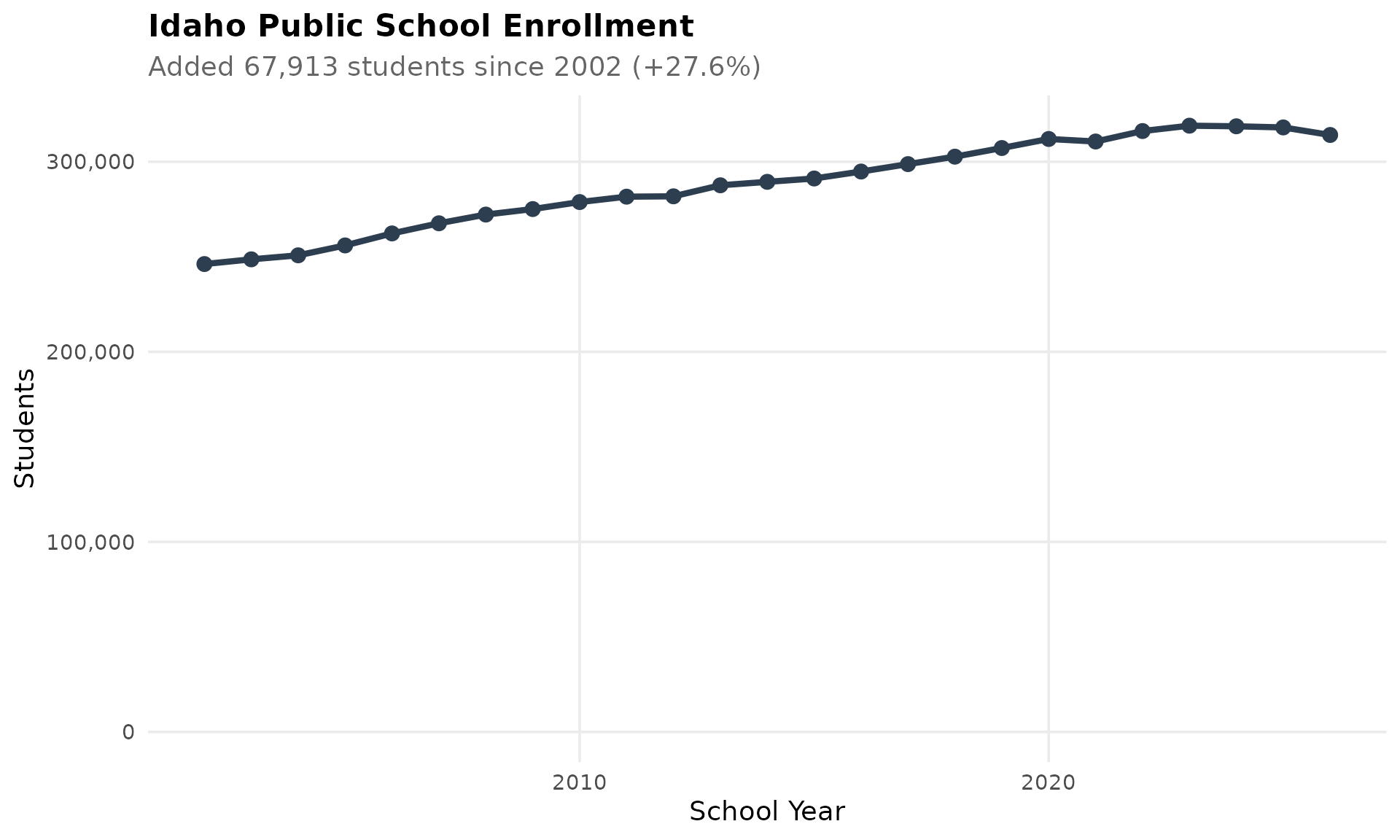
2. Boise proper declined while suburbs exploded
Boise Independent School District has declined to 22,000 students. Meanwhile, neighboring West Ada has grown from 20,000 to nearly 38,000. The growth is all in the suburbs.
boise_westada <- enr_all %>%
  filter(is_district,
         grepl("^BOISE INDEPENDENT DISTRICT|^WEST ADA DISTRICT", district_name),
         subgroup == "total_enrollment", grade_level == "TOTAL")
stopifnot(nrow(boise_westada) > 0)
boise_westada %>% select(end_year, district_name, n_students)
#>    end_year              district_name n_students
#> 1      2002 BOISE INDEPENDENT DISTRICT      25553
#> 2      2002          WEST ADA DISTRICT      21474
#> ...
#> 49     2026 BOISE INDEPENDENT DISTRICT      21717
#> 50     2026          WEST ADA DISTRICT      37919

ggplot(boise_westada, aes(x = end_year, y = n_students, color = district_name)) +
  geom_line(linewidth = 1.2) +
  geom_point(size = 2.5) +
  scale_y_continuous(labels = comma) +
  scale_color_manual(values = c(colors["district1"], colors["district2"])) +
  labs(title = "Boise Flat, West Ada Exploding",
       subtitle = "Suburban growth outpacing the urban core",
       x = "School Year", y = "Students", color = "") +
  theme_readme()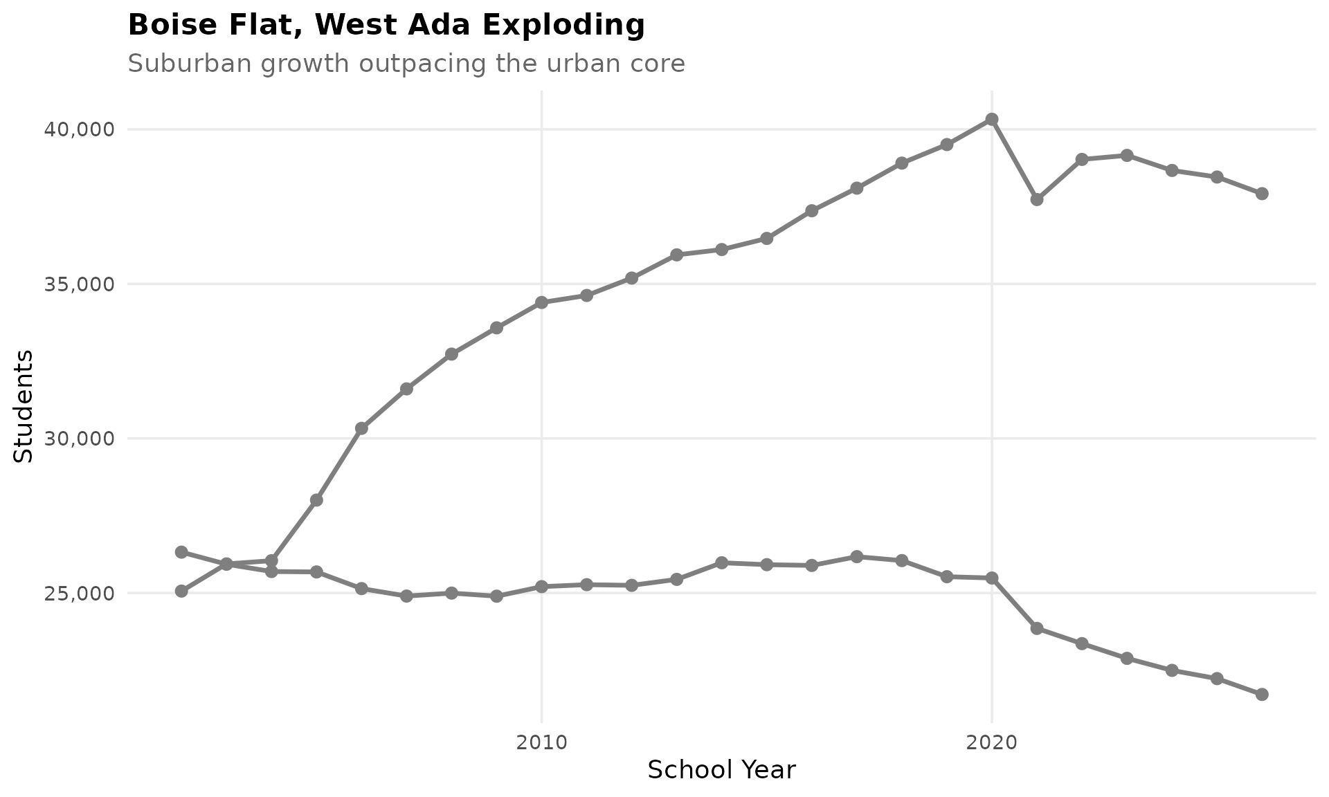
3. COVID barely slowed Idaho
Most states lost 3-5% enrollment during the pandemic. Idaho dipped briefly in 2020, then resumed growing. Families moved TO Idaho during the pandemic, offsetting any losses.
covid_years <- enr_all %>%
  filter(is_state, grade_level == "TOTAL", subgroup == "total_enrollment",
         end_year >= 2018)
stopifnot(nrow(covid_years) > 0)
covid_years %>% select(end_year, n_students)
#>   end_year n_students
#> 1     2018     302689
#> 2     2019     307228
#> 3     2020     311991
#> 4     2021     310653
#> 5     2022     316159
#> 6     2023     318979
#> 7     2024     318660
#> 8     2025     318067
#> 9     2026     314097

ggplot(covid_years, aes(x = end_year, y = n_students)) +
  geom_line(linewidth = 1.5, color = colors["total"]) +
  geom_point(size = 3, color = colors["total"]) +
  geom_vline(xintercept = 2021, linetype = "dashed", color = "red", alpha = 0.5) +
  annotate("text", x = 2021.3, y = max(covid_years$n_students, na.rm = TRUE) * 0.98,
           label = "COVID", hjust = 0, color = "red") +
  scale_y_continuous(labels = comma, limits = c(0, NA)) +
  labs(title = "Idaho Barely Slowed During COVID",
       subtitle = "Brief dip before resuming growth (2020-21 marked)",
       x = "School Year", y = "Students") +
  theme_readme()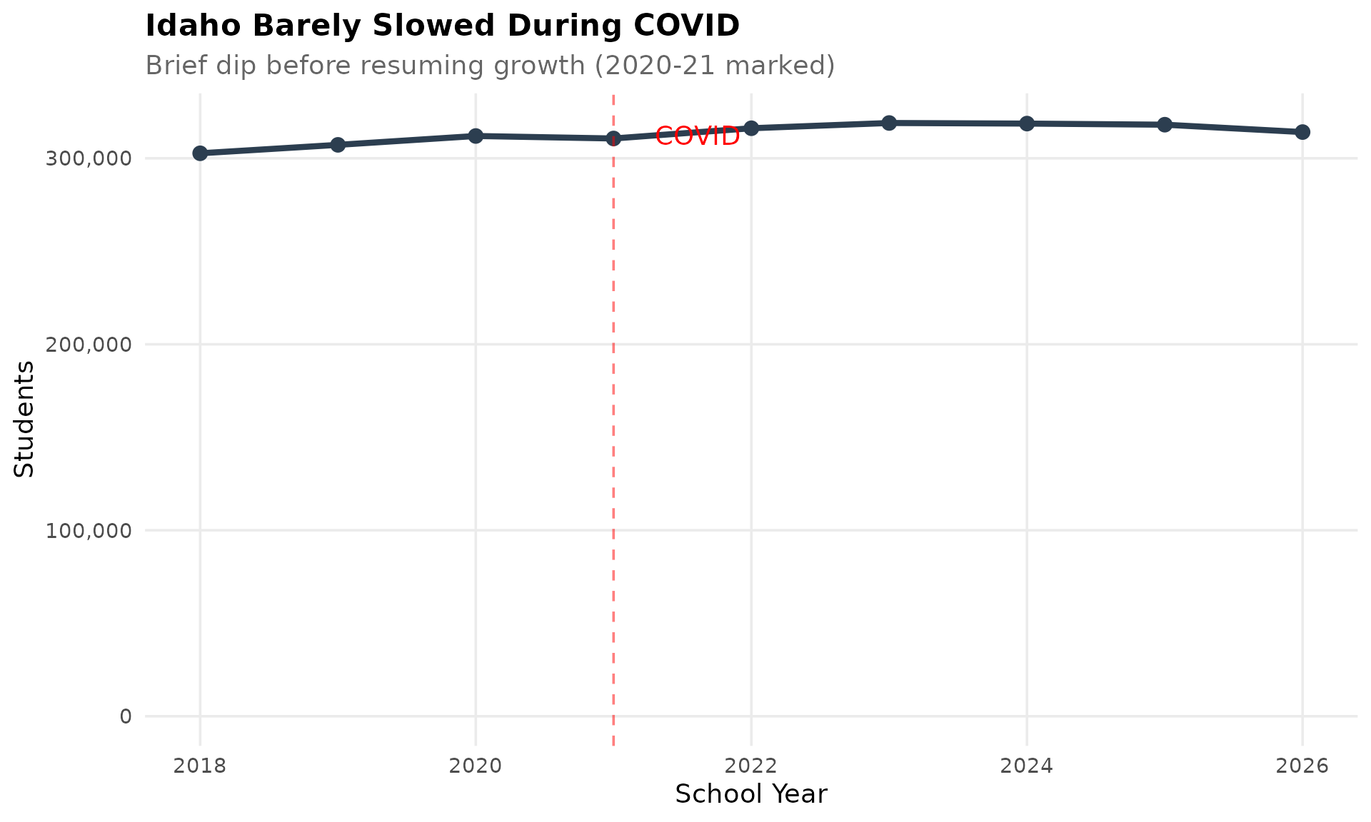
Data Taxonomy
| Category | Years | Function | Details |
|---|---|---|---|
| Enrollment | 1995-2026 |
fetch_enr() / fetch_enr_multi()
|
Grade-level (PK-12) by district/charter. Subgroups: total_enrollment. Entity flags: is_state, is_district, is_campus, is_charter. |
| Assessments | — | — | Not yet available |
| Graduation | — | — | Not yet available |
| Directory | 2011-2026 | fetch_directory() |
Building-level. District, charter status, grades served, school level, enrollment. |
| Per-Pupil Spending | — | — | Not yet available |
| Accountability | — | — | Not yet available |
| Chronic Absence | — | — | Not yet available |
| EL Progress | — | — | Not yet available |
| Special Ed | — | — | Not yet available |
See DATA-CATEGORY-TAXONOMY.md for what each category covers.
Quick Start
Installation
# install.packages("remotes")
remotes::install_github("almartin82/idschooldata")
R
library(idschooldata)
library(dplyr)

# Fetch one year
enr_2026 <- fetch_enr(2026)

# Fetch multiple years
enr_recent <- fetch_enr_multi(2020:2026)

# Fetch all available years
enr_all <- fetch_enr_multi(1996:2026)

# State totals
enr_2026 %>%
  filter(is_state, subgroup == "total_enrollment", grade_level == "TOTAL")

# District breakdown
enr_2026 %>%
  filter(is_district, subgroup == "total_enrollment", grade_level == "TOTAL") %>%
  arrange(desc(n_students))

# Grade-level breakdown
enr_2026 %>%
  filter(is_state, subgroup == "total_enrollment",
         grade_level %in% c("K", "01", "02", "03", "04", "05")) %>%
  select(grade_level, n_students)
Python
import pyidschooldata as id_

# Check available years
years = id_.get_available_years()
print(f"Data available from {years['min_year']} to {years['max_year']}")

# Fetch one year
enr_2026 = id_.fetch_enr(2026)

# Fetch multiple years
enr_recent = id_.fetch_enr_multi([2020, 2021, 2022, 2023, 2024, 2025, 2026])

# State totals
state_total = enr_2026[
    (enr_2026['is_state'] == True) &
    (enr_2026['subgroup'] == 'total_enrollment') &
    (enr_2026['grade_level'] == 'TOTAL')
]

# District breakdown
districts = enr_2026[
    (enr_2026['is_district'] == True) &
    (enr_2026['subgroup'] == 'total_enrollment') &
    (enr_2026['grade_level'] == 'TOTAL')
].sort_values('n_students', ascending=False)
Explore More
- Full documentation — all 15 stories with interactive charts
- Function reference
Data Notes
| Years | Source | Aggregation Levels | Notes |
|---|---|---|---|
| 1996-2026 | Idaho SDE Finance Portal | State, District, Charter | Grade-level breakdowns for all years |
What’s available
- Levels: State, district (~115), charter (~32)
- Grade levels: Preschool through Grade 12
- Years: 30 years of historical data
- Suppression: Idaho SDE does not suppress enrollment counts in this dataset
ID System
Idaho uses a 3-digit district numbering system: - District ID: 3 digits (e.g., 001 for Boise) - Charter IDs: Higher numbers in the 400+ series
Demographics Note
Race/ethnicity and special population data (ELL, Special Ed) are available through the Idaho Report Card but not included in the main enrollment file. This package focuses on the comprehensive grade-level enrollment data from the SDE Finance Portal.
Deeper Dive
4. West Ada is Idaho’s school giant
West Ada School District in suburban Boise (Meridian/Eagle area) serves nearly 38,000 students - 75% larger than Boise itself. It’s the largest district in the state and still growing.
top_10 <- enr_current %>%
  filter(is_district, grade_level == "TOTAL", subgroup == "total_enrollment") %>%
  arrange(desc(n_students)) %>%
  head(10)
stopifnot(nrow(top_10) > 0)

# Compute ratio dynamically
west_ada <- top_10$n_students[1]
boise <- top_10$n_students[top_10$district_name == "BOISE INDEPENDENT DISTRICT"]
ratio_pct <- round((west_ada / boise - 1) * 100)

top_10 %>% select(district_name, n_students)
#>                          district_name n_students
#> 1                    WEST ADA DISTRICT      37919
#> 2           BOISE INDEPENDENT DISTRICT      21717
#> 3            BONNEVILLE JOINT DISTRICT      13511
#> 4                NAMPA SCHOOL DISTRICT      12473
#> 5                   POCATELLO DISTRICT      11437
#> 6             VALLIVUE SCHOOL DISTRICT      10700
#> 7                 IDAHO FALLS DISTRICT       9751
#> 8               COEUR D ALENE DISTRICT       9680
#> 9                  TWIN FALLS DISTRICT       8774
#> 10 IDAHO HOME LEARNING ACADEMY CHARTER       7504

ggplot(top_10, aes(x = reorder(district_name, n_students), y = n_students)) +
  geom_col(fill = colors["total"]) +
  coord_flip() +
  scale_y_continuous(labels = comma) +
  labs(title = "Idaho's Largest School Districts",
       subtitle = paste0("West Ada serves ", ratio_pct, "% more students than Boise"),
       x = "", y = "Students") +
  theme_readme()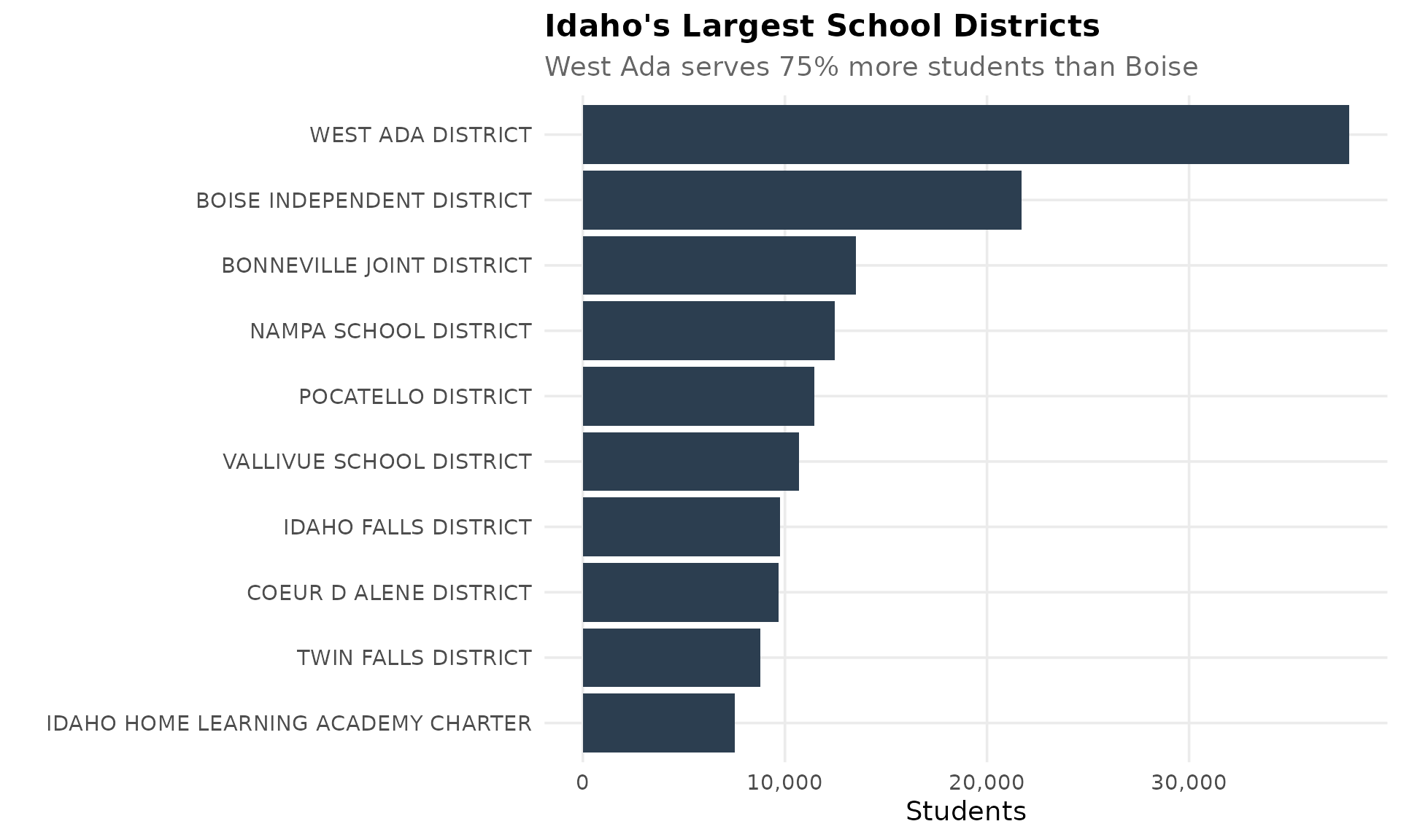
5. The Treasure Valley boom
Eagle, Kuna, Star, and Middleton are among the fastest-growing communities in America. These districts around Boise have doubled or tripled enrollment in 15 years as families flee California.
treasure_valley <- c("WEST ADA DISTRICT", "KUNA JOINT DISTRICT", "MIDDLETON DISTRICT")
tv_trend <- enr_decade %>%
  filter(is_district,
         grepl(paste(treasure_valley, collapse = "|"), district_name),
         subgroup == "total_enrollment", grade_level == "TOTAL")
stopifnot(nrow(tv_trend) > 0)
tv_trend %>% select(end_year, district_name, n_students)
#>    end_year       district_name n_students
#> 1      2012   WEST ADA DISTRICT      35188
#> 2      2012 KUNA JOINT DISTRICT       4983
#> 3      2012  MIDDLETON DISTRICT       3219
#> ...
#> 43     2026   WEST ADA DISTRICT      37919
#> 44     2026 KUNA JOINT DISTRICT       5699
#> 45     2026  MIDDLETON DISTRICT       4401

ggplot(tv_trend, aes(x = end_year, y = n_students, color = district_name)) +
  geom_line(linewidth = 1.2) +
  geom_point(size = 2.5) +
  scale_y_continuous(labels = comma) +
  scale_color_manual(values = c(colors["district1"], colors["district2"], colors["district3"])) +
  labs(title = "Treasure Valley Suburban Growth",
       subtitle = "West Ada, Kuna, and Middleton growing rapidly",
       x = "School Year", y = "Students", color = "") +
  theme_readme()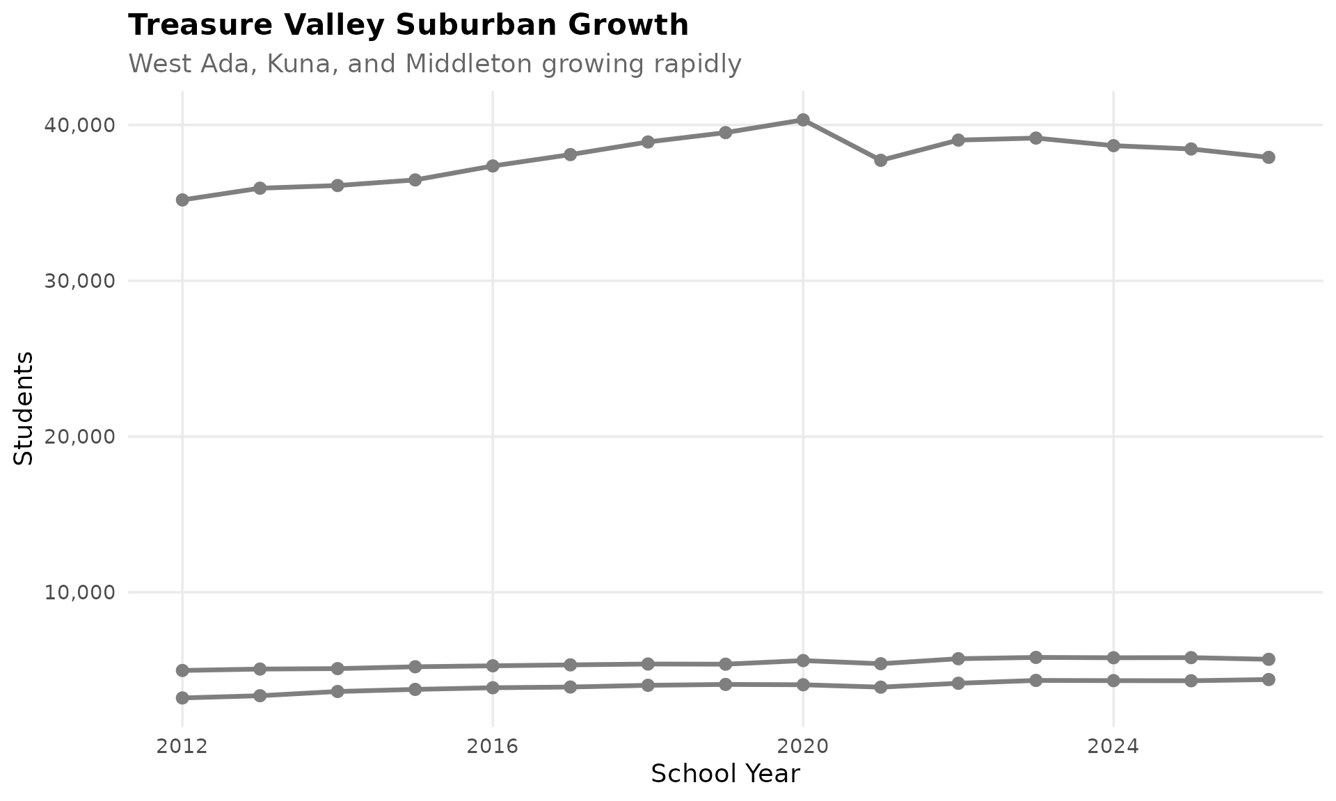
6. Kindergarten enrollment follows national trends
Like most states, Idaho’s kindergarten enrollment has declined in recent years as birth rates drop statewide. The decline appears to have stabilized since 2021.
k_trend <- enr_decade %>%
  filter(is_state, subgroup == "total_enrollment", grade_level == "K")
stopifnot(nrow(k_trend) > 0)
k_trend %>% select(end_year, n_students)
#>    end_year n_students
#> 1      2012      23038
#> 2      2013      23765
#> ...
#> 14     2025      22544
#> 15     2026      22154

ggplot(k_trend, aes(x = end_year, y = n_students)) +
  geom_line(linewidth = 1.5, color = colors["growth"]) +
  geom_point(size = 3, color = colors["growth"]) +
  scale_y_continuous(labels = comma) +
  labs(title = "Idaho Kindergarten Enrollment",
       subtitle = "Decline stabilized since 2021",
       x = "School Year", y = "Students") +
  theme_readme()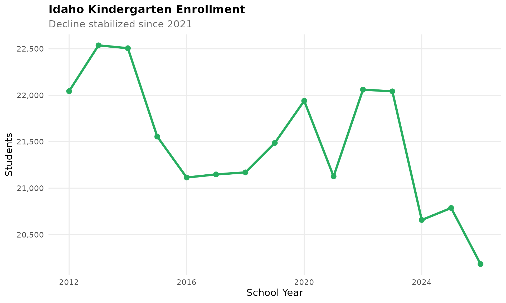
7. Charter schools serve 1 in 14 Idaho students
Idaho has 32 charter schools serving nearly 23,000 students. Idaho Home Learning Academy alone accounts for over 7,500 students - a third of all charter enrollment.
charter <- enr_current %>%
  filter(is_charter, grade_level == "TOTAL", subgroup == "total_enrollment")
stopifnot(nrow(charter) > 0)

charter_total <- sum(charter$n_students, na.rm = TRUE)
state_total <- enr_current %>%
  filter(is_state, grade_level == "TOTAL", subgroup == "total_enrollment") %>%
  pull(n_students)
charter_ratio <- round(state_total / charter_total)

charter %>%
  arrange(desc(n_students)) %>%
  head(10) %>%
  select(district_name, n_students)
#>                          district_name n_students
#> 1  IDAHO HOME LEARNING ACADEMY CHARTER       7504
#> 2          INSPIRE VIRTUAL CHARTER LEA       1553
#> 3                   IDAHO ARTS CHARTER       1421
#> 4         COMPAS PUBLIC CHARTER SCHOOL       1289
#> 5                   NORTH STAR CHARTER       1143
#> 6                VISION CHARTER SCHOOL        757
#> 7                XAVIER CHARTER SCHOOL        675
#> 8            WHITE PINE CHARTER SCHOOL        653
#> 9                 ANSER CHARTER SCHOOL        598
#> 10       COEUR D'ALENE CHARTER ACADEMY        593

charter %>%
  arrange(desc(n_students)) %>%
  head(10) %>%
  ggplot(aes(x = reorder(district_name, n_students), y = n_students)) +
  geom_col(fill = colors["district3"]) +
  coord_flip() +
  scale_y_continuous(labels = comma) +
  labs(title = "Idaho's Largest Charter Schools",
       subtitle = paste0(format(charter_total, big.mark = ","),
                        " students in charters (",
                        round(charter_total / state_total * 100, 1),
                        "% of state, 1 in ", charter_ratio, ")"),
       x = "", y = "Students") +
  theme_readme()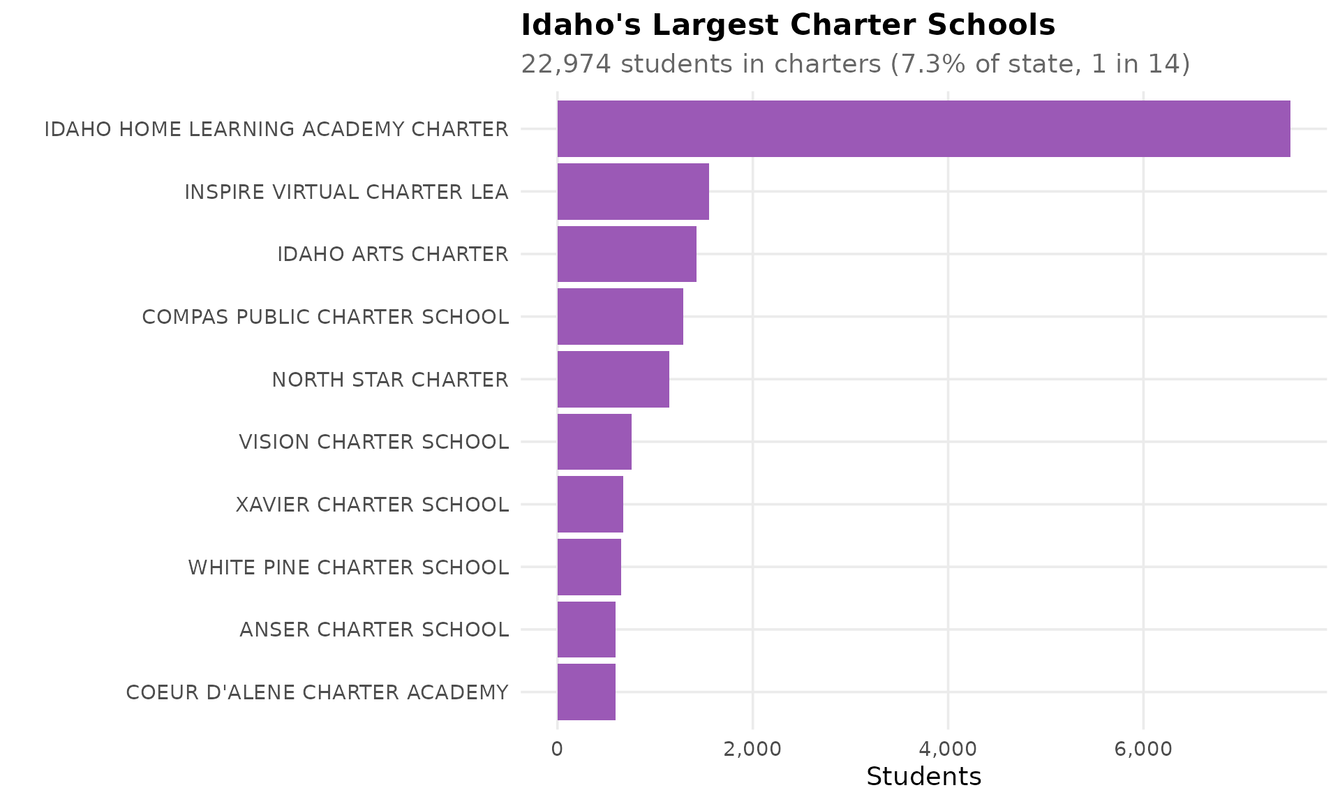
8. Rural Idaho is emptying out
While Boise suburbs boom, northern and eastern Idaho are hollowing out. Wallace (Silver Valley), Salmon, and Challis have lost half their students in 20 years.
rural <- c("WALLACE DISTRICT", "SALMON DISTRICT", "CHALLIS JOINT DISTRICT")
rural_trend <- enr_all %>%
  filter(is_district,
         grepl(paste(rural, collapse = "|"), district_name),
         subgroup == "total_enrollment", grade_level == "TOTAL")
stopifnot(nrow(rural_trend) > 0)
rural_trend %>% select(end_year, district_name, n_students)
#>    end_year          district_name n_students
#> 1      2002    CHALLIS JOINT DISTRICT        647
#> 2      2002         SALMON DISTRICT        852
#> 3      2002        WALLACE DISTRICT        579
#> ...

ggplot(rural_trend, aes(x = end_year, y = n_students, color = district_name)) +
  geom_line(linewidth = 1.2) +
  geom_point(size = 2) +
  scale_y_continuous(labels = comma) +
  scale_color_manual(values = c(colors["decline"], colors["district2"], colors["district3"])) +
  labs(title = "Rural Idaho is Emptying Out",
       subtitle = "Northern mountain communities losing students",
       x = "School Year", y = "Students", color = "") +
  theme_readme()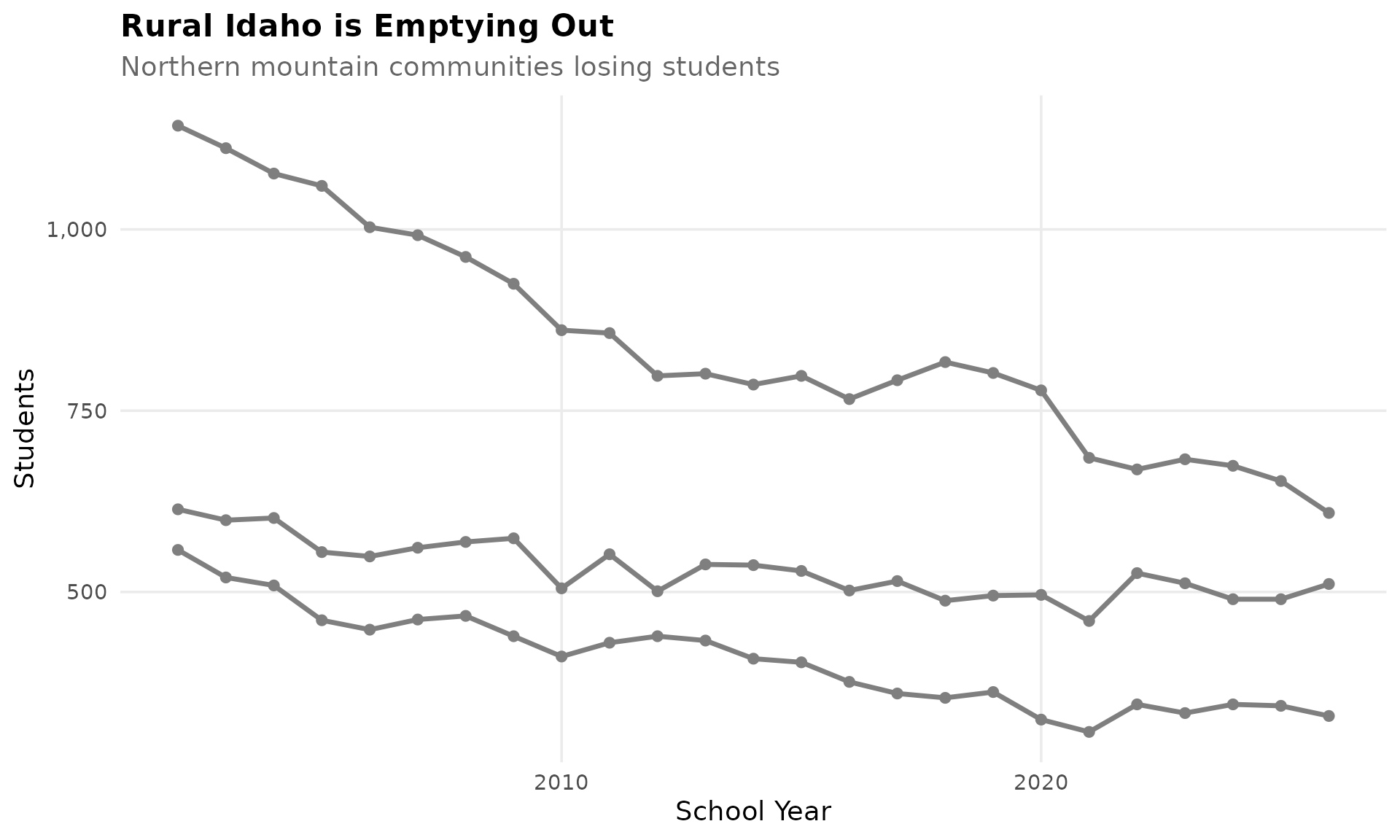
9. High school enrollment surged 22% in 15 years
Idaho’s high schools are seeing record enrollment as the wave of growth works through the grades.
hs_trend <- enr_decade %>%
  filter(is_state, subgroup == "total_enrollment",
         grade_level %in% c("09", "10", "11", "12")) %>%
  group_by(end_year) %>%
  summarize(n_students = sum(n_students, na.rm = TRUE), .groups = "drop")
stopifnot(nrow(hs_trend) > 0)

# Compute growth dynamically
hs_first <- hs_trend$n_students[1]
hs_last <- hs_trend$n_students[nrow(hs_trend)]
hs_pct <- round((hs_last / hs_first - 1) * 100)

hs_trend
#> # A tibble: 15 x 2
#>    end_year n_students
#>       <dbl>      <dbl>
#>  1     2012      83121
#>  2     2013      83952
#> ...
#> 14     2025     102039
#> 15     2026     101402
cat("HS growth:", format(hs_first, big.mark = ","), "->",
    format(hs_last, big.mark = ","), "(+", hs_pct, "%)\n")
#> HS growth: 83,121 -> 101,402 (+ 22 %)

ggplot(hs_trend, aes(x = end_year, y = n_students)) +
  geom_line(linewidth = 1.5, color = colors["total"]) +
  geom_point(size = 3, color = colors["total"]) +
  scale_y_continuous(labels = comma, limits = c(0, NA)) +
  labs(title = "Idaho High School Enrollment (Grades 9-12)",
       subtitle = paste0("From ", format(hs_first, big.mark = ","), " to ",
                        format(hs_last, big.mark = ","), " (+", hs_pct, "%)"),
       x = "School Year", y = "Students") +
  theme_readme()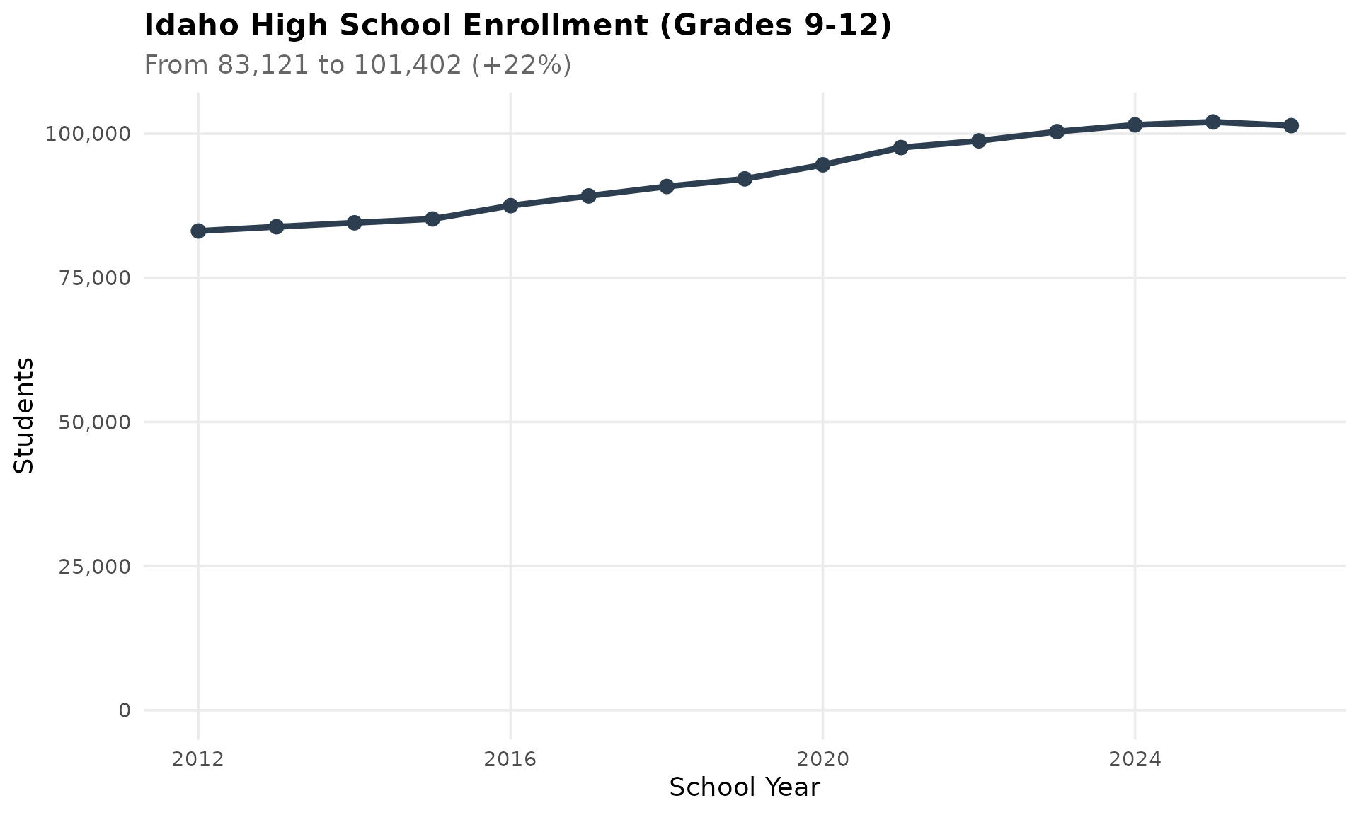
10. The Magic Valley is holding steady
Twin Falls, Jerome, and Minidoka County in south-central Idaho have maintained steady enrollment even as some rural areas shrink. Agriculture and food processing anchor these communities.
magic_valley <- c("TWIN FALLS DISTRICT", "JEROME JOINT DISTRICT", "MINIDOKA COUNTY JOINT DISTRICT")
mv_trend <- enr_decade %>%
  filter(is_district,
         grepl(paste(magic_valley, collapse = "|"), district_name),
         !grepl("VIRTUAL|CHARTER", district_name),
         subgroup == "total_enrollment", grade_level == "TOTAL")
stopifnot(nrow(mv_trend) > 0)
mv_trend %>% select(end_year, district_name, n_students)
#>    end_year                  district_name n_students
#> 1      2012 MINIDOKA COUNTY JOINT DISTRICT       4320
#> 2      2012          TWIN FALLS DISTRICT       8147
#> 3      2012       JEROME JOINT DISTRICT       3860
#> ...

ggplot(mv_trend, aes(x = end_year, y = n_students, color = district_name)) +
  geom_line(linewidth = 1.2) +
  geom_point(size = 2.5) +
  scale_y_continuous(labels = comma) +
  scale_color_manual(values = c(colors["district1"], colors["district2"], colors["district3"])) +
  labs(title = "Magic Valley Districts Holding Steady",
       subtitle = "Twin Falls and Jerome maintain enrollment",
       x = "School Year", y = "Students", color = "") +
  theme_readme()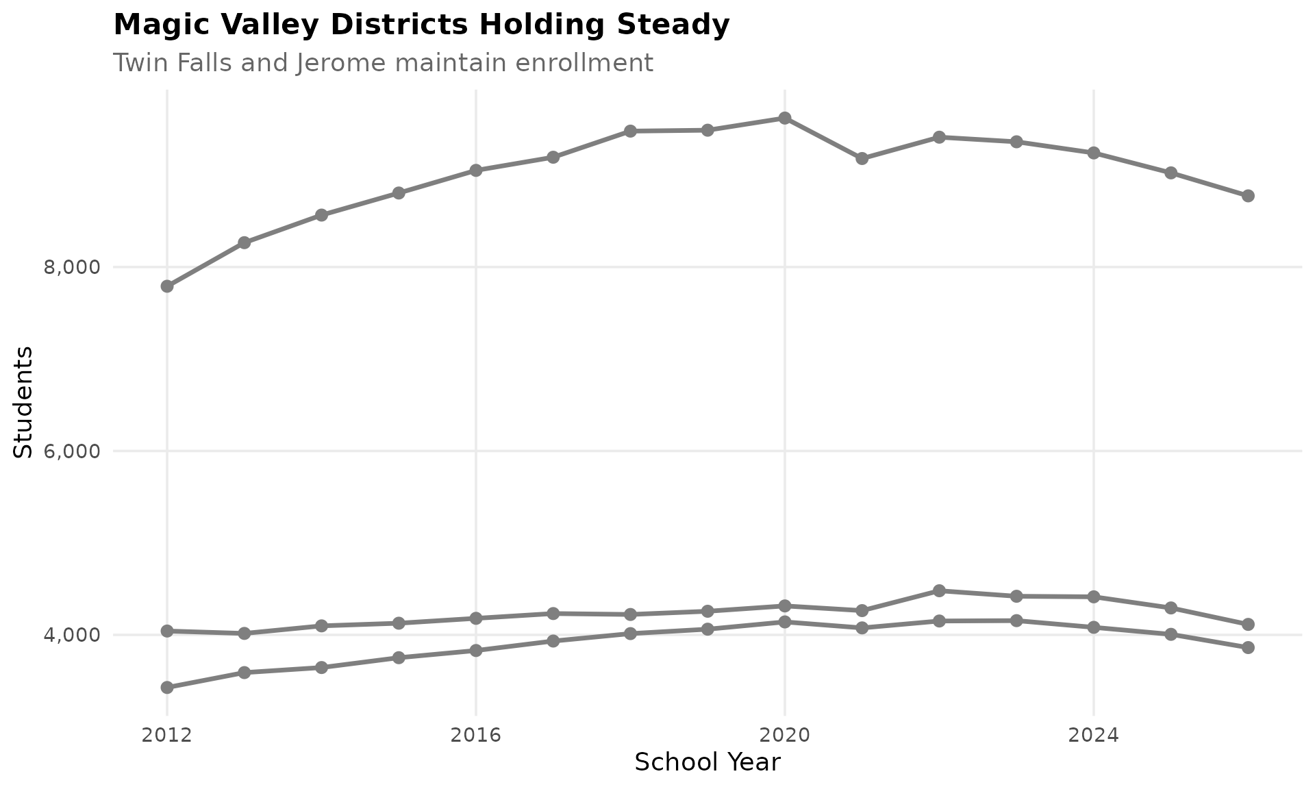
11. Elementary is the biggest cohort
Idaho’s elementary schools (K-5) serve the largest share of students. The grade distribution shows a healthy pipeline with growing younger grades - a sign of continued future growth.
grades <- enr_current %>%
  filter(is_state, subgroup == "total_enrollment",
         grade_level %in% c("K", "01", "02", "03", "04", "05",
                           "06", "07", "08", "09", "10", "11", "12"))
stopifnot(nrow(grades) > 0)

grade_order <- c("K", "01", "02", "03", "04", "05",
                 "06", "07", "08", "09", "10", "11", "12")
grades$grade_level <- factor(grades$grade_level, levels = grade_order)

grades %>% select(grade_level, n_students)
#>    grade_level n_students
#> 1            K      22154
#> 2           01      22781
#> 3           02      23230
#> 4           03      23578
#> 5           04      23636
#> 6           05      24017
#> 7           06      24082
#> 8           07      24543
#> 9           08      24576
#> 10          09      26429
#> 11          10      26003
#> 12          11      25117
#> 13          12      23864

ggplot(grades, aes(x = grade_level, y = n_students)) +
  geom_col(fill = colors["total"]) +
  scale_y_continuous(labels = comma) +
  labs(title = "Idaho Enrollment by Grade Level",
       subtitle = "Strong elementary enrollment signals continued growth",
       x = "Grade", y = "Students") +
  theme_readme()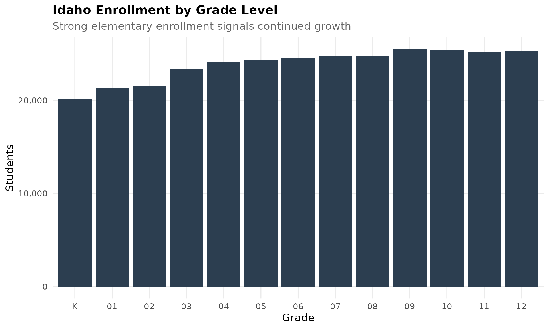
12. Coeur d’Alene leads northern Idaho
In the Idaho panhandle, Coeur d’Alene School District leads with nearly 10,000 students. Post Falls and Lakeland are also growing as people relocate from Spokane and beyond.
north <- c("COEUR D ALENE DISTRICT", "POST FALLS DISTRICT", "LAKELAND DISTRICT")
north_trend <- enr_decade %>%
  filter(is_district,
         grepl(paste(north, collapse = "|"), district_name),
         subgroup == "total_enrollment", grade_level == "TOTAL")
stopifnot(nrow(north_trend) > 0)
north_trend %>% select(end_year, district_name, n_students)
#>    end_year          district_name n_students
#> 1      2012 COEUR D ALENE DISTRICT       9903
#> 2      2012    POST FALLS DISTRICT       5133
#> 3      2012      LAKELAND DISTRICT       4061
#> ...

ggplot(north_trend, aes(x = end_year, y = n_students, color = district_name)) +
  geom_line(linewidth = 1.2) +
  geom_point(size = 2.5) +
  scale_y_continuous(labels = comma) +
  scale_color_manual(values = c(colors["district1"], colors["district2"], colors["district3"])) +
  labs(title = "North Idaho District Growth",
       subtitle = "Coeur d'Alene, Post Falls, and Lakeland expanding",
       x = "School Year", y = "Students", color = "") +
  theme_readme()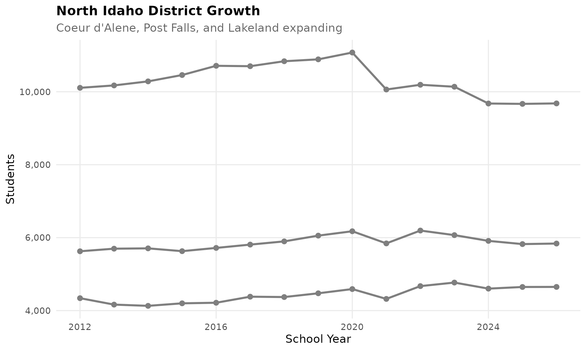
13. Small districts dominate the landscape
Idaho has 115+ school districts, but many are tiny. Over 40 districts have fewer than 500 students. These small rural districts face unique challenges with limited resources.
district_sizes <- enr_current %>%
  filter(is_district, grade_level == "TOTAL", subgroup == "total_enrollment") %>%
  mutate(size_category = case_when(
    n_students >= 10000 ~ "10,000+",
    n_students >= 5000 ~ "5,000-9,999",
    n_students >= 2000 ~ "2,000-4,999",
    n_students >= 1000 ~ "1,000-1,999",
    n_students >= 500 ~ "500-999",
    TRUE ~ "Under 500"
  )) %>%
  group_by(size_category) %>%
  summarize(n_districts = n(), .groups = "drop")
stopifnot(nrow(district_sizes) > 0)

district_sizes$size_category <- factor(district_sizes$size_category,
  levels = c("Under 500", "500-999", "1,000-1,999", "2,000-4,999", "5,000-9,999", "10,000+"))

district_sizes
#>   size_category n_districts
#> 1     Under 500          56
#> 2       500-999          26
#> 3   1,000-1,999          16
#> 4   2,000-4,999           9
#> 5   5,000-9,999           4
#> 6       10,000+           6

ggplot(district_sizes, aes(x = size_category, y = n_districts)) +
  geom_col(fill = colors["total"]) +
  labs(title = "Idaho Districts by Size",
       subtitle = "Many small rural districts, few large ones",
       x = "District Size (Students)", y = "Number of Districts") +
  theme_readme()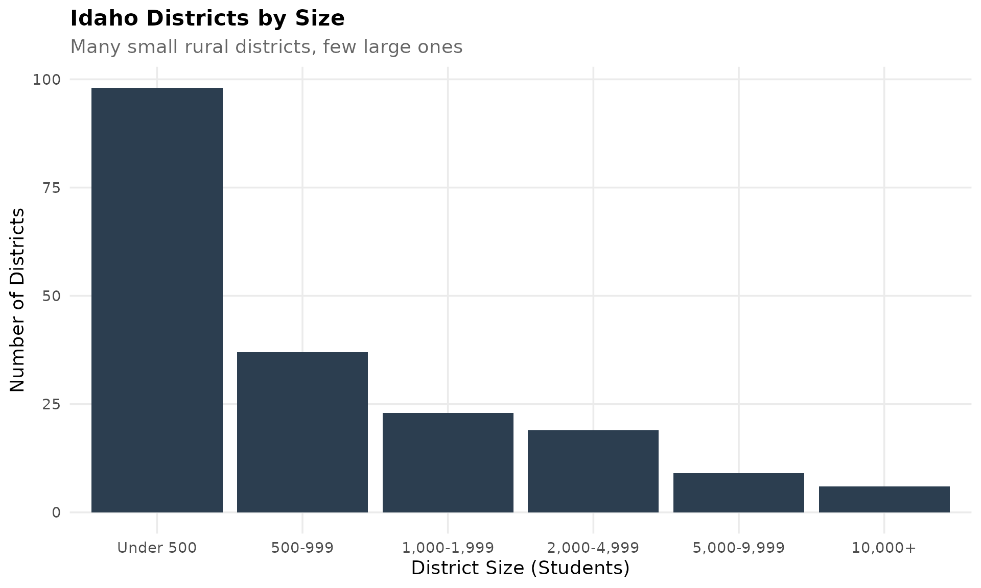
14. Nampa and Caldwell anchor Canyon County
Nampa School District and Caldwell serve Canyon County west of Boise. Both have grown with the Treasure Valley, though Nampa has seen recent declines from its 2014 peak.
canyon <- c("NAMPA SCHOOL DISTRICT", "CALDWELL DISTRICT")
canyon_trend <- enr_decade %>%
  filter(is_district,
         grepl(paste(canyon, collapse = "|"), district_name),
         subgroup == "total_enrollment", grade_level == "TOTAL")
stopifnot(nrow(canyon_trend) > 0)
canyon_trend %>% select(end_year, district_name, n_students)
#>    end_year      district_name n_students
#> 1      2012 NAMPA SCHOOL DISTRICT      13376
#> 2      2012    CALDWELL DISTRICT       6124
#> ...

ggplot(canyon_trend, aes(x = end_year, y = n_students, color = district_name)) +
  geom_line(linewidth = 1.2) +
  geom_point(size = 2.5) +
  scale_y_continuous(labels = comma) +
  scale_color_manual(values = c(colors["district1"], colors["district2"])) +
  labs(title = "Canyon County Districts",
       subtitle = "Nampa and Caldwell growing with Treasure Valley",
       x = "School Year", y = "Students", color = "") +
  theme_readme()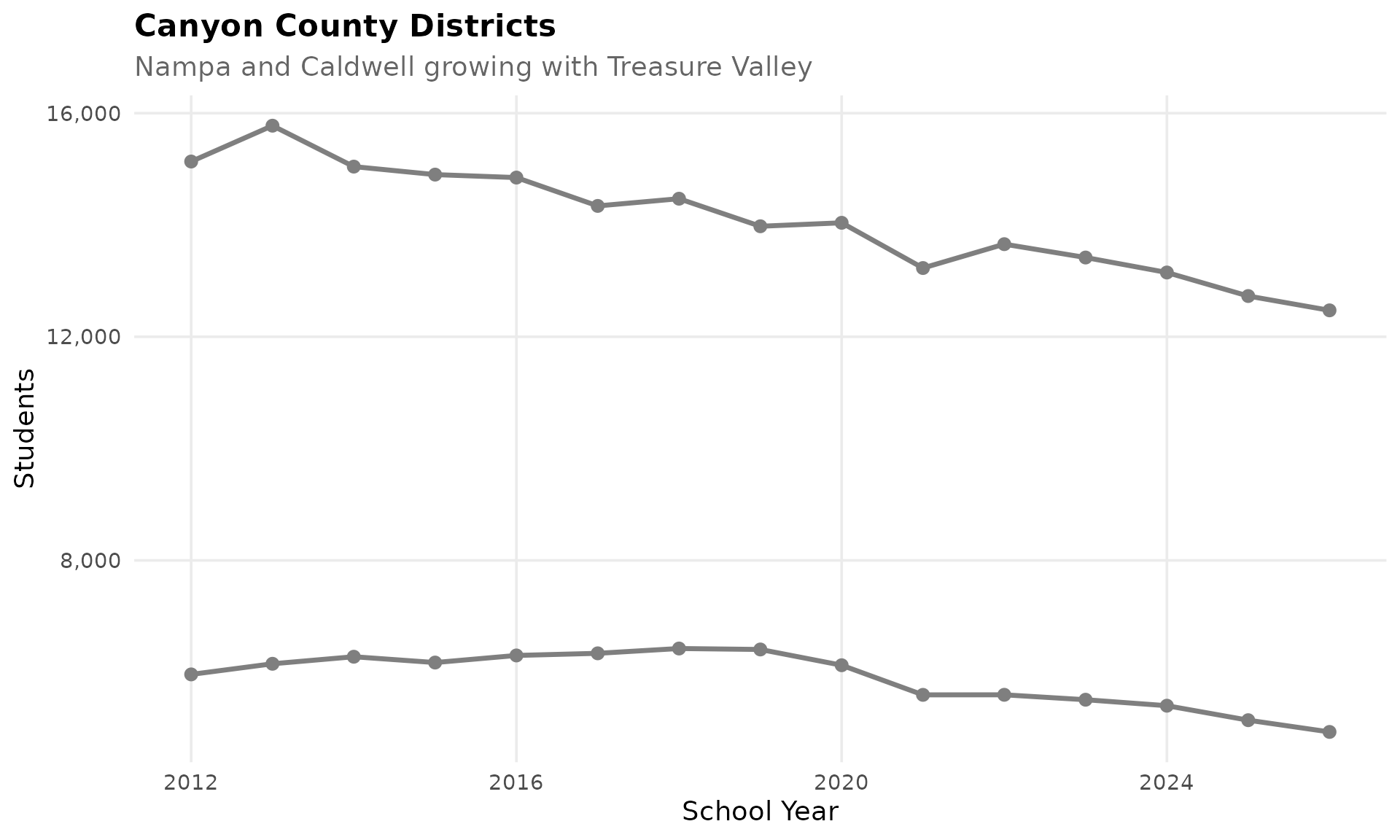
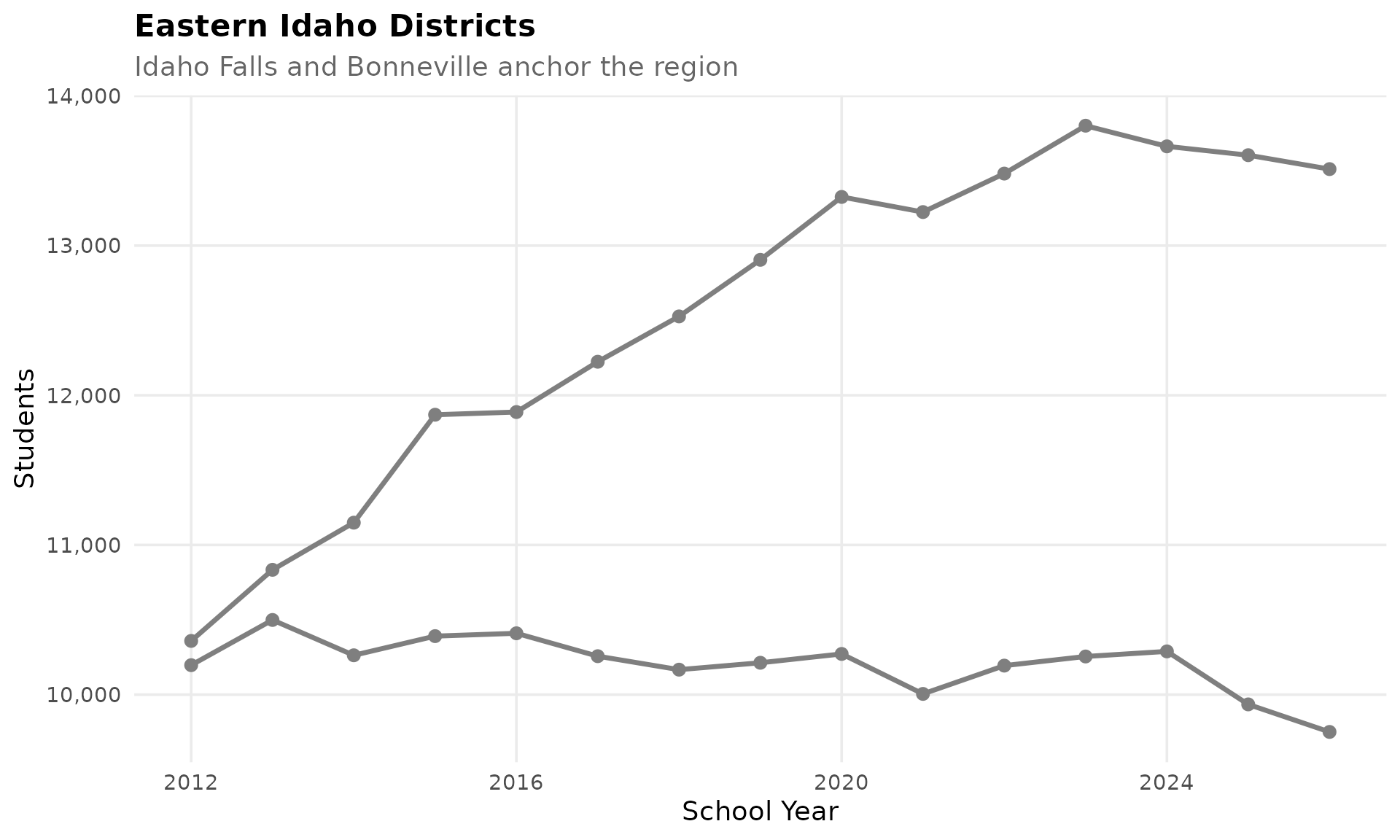
15. Idaho Falls leads eastern Idaho
Idaho Falls School District (#91) anchors the eastern region with nearly 10,000 students. Nearby Bonneville Joint District serves the growing suburban areas with 13,500 students. Eastern Idaho grows more slowly than the Treasure Valley.
eastern <- c("IDAHO FALLS DISTRICT", "BONNEVILLE JOINT DISTRICT")
eastern_trend <- enr_decade %>%
  filter(is_district,
         grepl(paste(eastern, collapse = "|"), district_name),
         subgroup == "total_enrollment", grade_level == "TOTAL")
stopifnot(nrow(eastern_trend) > 0)
eastern_trend %>% select(end_year, district_name, n_students)
#>    end_year              district_name n_students
#> 1      2012 BONNEVILLE JOINT DISTRICT      11827
#> 2      2012      IDAHO FALLS DISTRICT       9282
#> ...

ggplot(eastern_trend, aes(x = end_year, y = n_students, color = district_name)) +
  geom_line(linewidth = 1.2) +
  geom_point(size = 2.5) +
  scale_y_continuous(labels = comma) +
  scale_color_manual(values = c(colors["district1"], colors["district2"])) +
  labs(title = "Eastern Idaho Districts",
       subtitle = "Idaho Falls and Bonneville anchor the region",
       x = "School Year", y = "Students", color = "") +
  theme_readme()