theme_readme <- function() {
  theme_minimal(base_size = 14) +
    theme(
      plot.title = element_text(face = "bold", size = 16),
      plot.subtitle = element_text(color = "gray40"),
      panel.grid.minor = element_blank(),
      legend.position = "bottom"
    )
}

colors <- c("total" = "#2C3E50", "white" = "#3498DB", "black" = "#E74C3C",
            "hispanic" = "#F39C12", "asian" = "#9B59B6")
# Get available years
years <- get_available_years()
max_year <- max(years)
min_year <- min(years)

# Fetch recent 10 years of data
enr <- fetch_enr_multi((max_year - 9):max_year, use_cache = TRUE)

# Fetch long-range milestone years
key_years <- c(2006, 2011, 2016, 2021, max_year)
key_years <- key_years[key_years >= min_year & key_years <= max_year]
enr_long <- fetch_enr_multi(key_years, use_cache = TRUE)

# Fetch current year data
enr_current <- fetch_enr(max_year, use_cache = TRUE)
1. Indiana lost 55,000 students since 2006
Indiana enrollment peaked above 1.08 million in 2006 and has steadily declined to just over 1.03 million. The state lost about 5% of its public school enrollment over two decades.
state_trend <- enr %>%
  filter(is_state, grade_level == "TOTAL", subgroup == "total_enrollment")

stopifnot(nrow(state_trend) > 0)

state_trend %>% select(end_year, n_students)
#>    end_year n_students
#> 1      2017    1049292
#> 2      2018    1053809
#> 3      2019    1055354
#> 4      2020    1051051
#> 5      2021    1033781
#> 6      2022    1036697
#> 7      2023    1036123
#> 8      2024    1032724
#> 9      2025    1040190
#> 10     2026    1028466

ggplot(state_trend, aes(x = end_year, y = n_students)) +
  geom_line(linewidth = 1.5, color = colors["total"]) +
  geom_point(size = 3, color = colors["total"]) +
  scale_y_continuous(labels = comma, limits = c(0, NA)) +
  labs(title = "Indiana Public School Enrollment",
       subtitle = "Gradual decline from 1.05M to 1.03M over the past decade",
       x = "School Year", y = "Students") +
  theme_readme()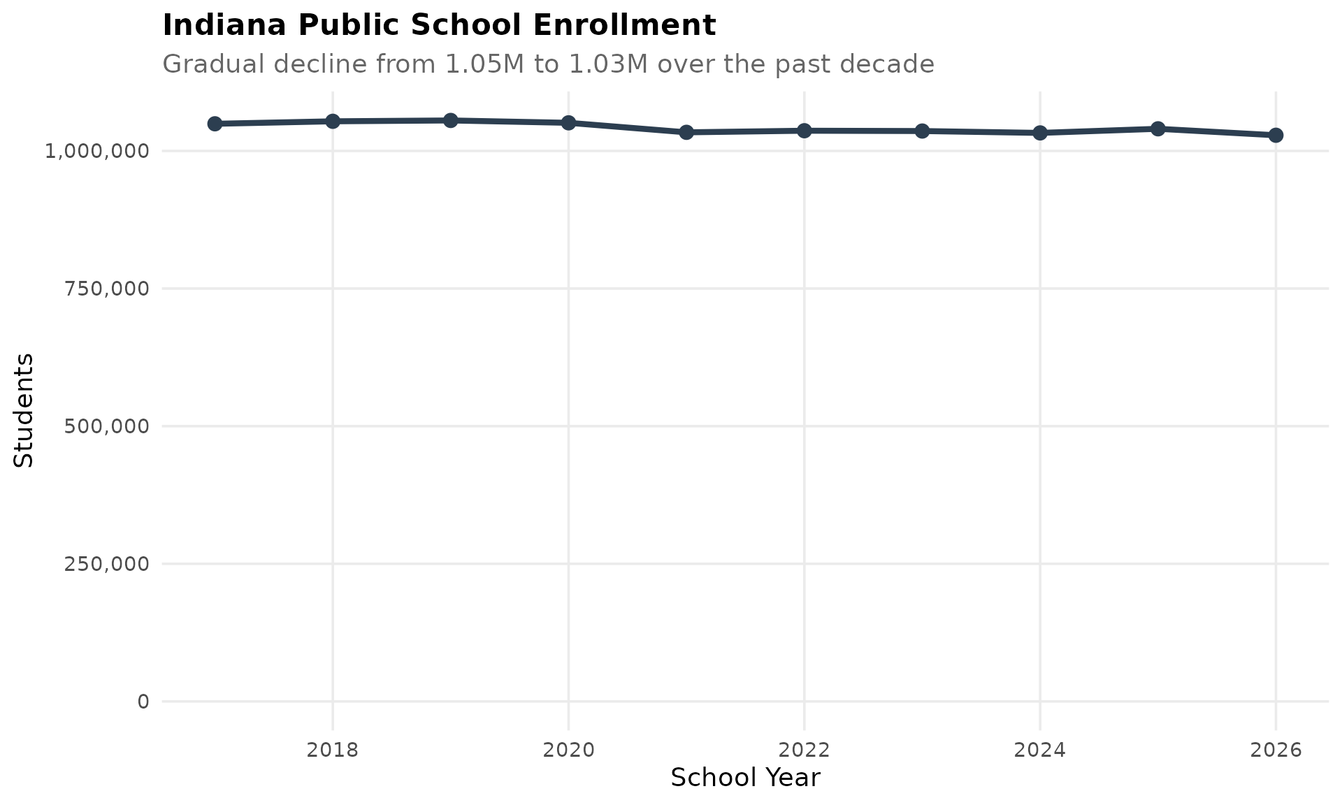
2. Indianapolis Public Schools has lost over 15,000 students
IPS enrollment dropped from 37,554 in 2006 to under 22,000 by 2024 – a 42% decline. Charter schools and suburban flight continue to reshape Indianapolis education.
ips <- enr_long %>%
  filter(is_corporation, grepl("Indianapolis Public Schools", corporation_name),
         subgroup == "total_enrollment", grade_level == "TOTAL")

stopifnot(nrow(ips) > 0)

ips %>% select(end_year, corporation_name, n_students)
#>   end_year            corporation_name n_students
#> 1     2006 Indianapolis Public Schools      37554
#> 2     2011 Indianapolis Public Schools      33080
#> 3     2016 Indianapolis Public Schools      29583
#> 4     2021 Indianapolis Public Schools      22930
#> 5     2026 Indianapolis Public Schools      19774

ggplot(ips, aes(x = end_year, y = n_students)) +
  geom_line(linewidth = 1.5, color = colors["total"]) +
  geom_point(size = 3, color = colors["total"]) +
  scale_y_continuous(labels = comma, limits = c(0, NA)) +
  labs(title = "Indianapolis Public Schools Decline",
       subtitle = "Lost over 15,000 students since 2006",
       x = "School Year", y = "Students") +
  theme_readme()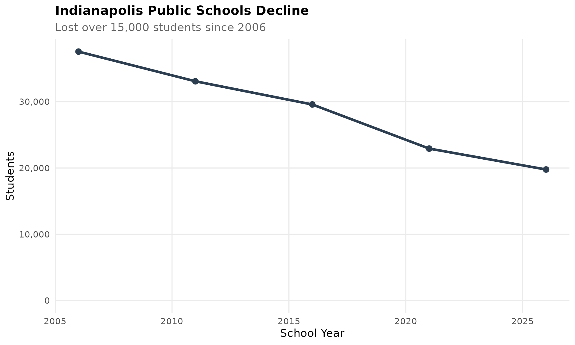
3. Hamilton County added 16,000 students since 2006
Carmel, Fishers, Westfield, and Noblesville suburbs are booming. These four Hamilton County corporations grew from about 42,000 to nearly 58,000 students – a 38% increase.
hamilton <- c("Carmel Clay Schools", "Hamilton Southeastern Schools",
              "Noblesville Schools", "Westfield-Washington Schools")

hamilton_trend <- enr %>%
  filter(corporation_name %in% hamilton, is_corporation,
         grade_level == "TOTAL", subgroup == "total_enrollment") %>%
  group_by(end_year) %>%
  summarize(total = sum(n_students, na.rm = TRUE), .groups = "drop")

stopifnot(nrow(hamilton_trend) > 0)

hamilton_trend
#> # A tibble: 10 × 2
#>    end_year total
#>       <int> <dbl>
#>  1     2017 55465
#>  2     2018 56306
#>  3     2019 56681
#>  4     2020 57958
#>  5     2021 57117
#>  6     2022 57281
#>  7     2023 57442
#>  8     2024 57687
#>  9     2025 57856
#> 10     2026 57290

ggplot(hamilton_trend, aes(x = end_year, y = total)) +
  geom_line(linewidth = 1.5, color = colors["total"]) +
  geom_point(size = 3, color = colors["total"]) +
  scale_y_continuous(labels = comma, limits = c(0, NA)) +
  labs(title = "Hamilton County: Indiana's Growth Engine",
       subtitle = "Carmel, Fishers, Noblesville, Westfield combined",
       x = "School Year", y = "Students") +
  theme_readme()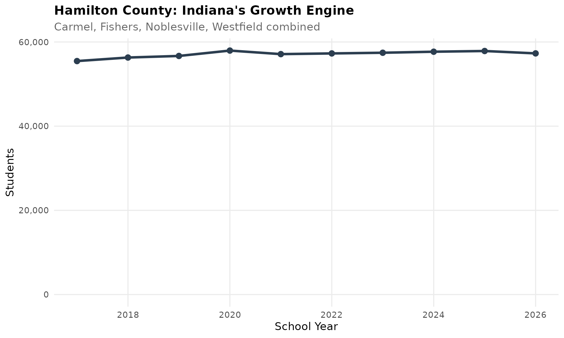
4. Hispanic enrollment has more than doubled
Hispanic students grew from 5.8% to 14.6% of enrollment since 2006, a 2.5x increase. Northwest Indiana and Indianapolis drive this demographic shift.
hispanic <- enr_long %>%
  filter(is_state, grade_level == "TOTAL", subgroup == "hispanic")

stopifnot(nrow(hispanic) > 0)

hispanic %>% select(end_year, n_students, pct) %>%
  mutate(pct_display = round(pct * 100, 1))
#>   end_year n_students        pct pct_display
#> 1     2006      62718 0.05765497         5.8
#> 2     2011      87790 0.08384341         8.4
#> 3     2016     116671 0.11148398        11.1
#> 4     2021     135497 0.13106935        13.1
#> 5     2026     158808 0.15441249        15.4

ggplot(hispanic, aes(x = end_year, y = pct * 100)) +
  geom_line(linewidth = 1.5, color = colors["hispanic"]) +
  geom_point(size = 3, color = colors["hispanic"]) +
  labs(title = "Hispanic Student Population in Indiana",
       subtitle = "More than doubled from 5.8% to 14.6% since 2006",
       x = "School Year", y = "Percent of Students") +
  theme_readme()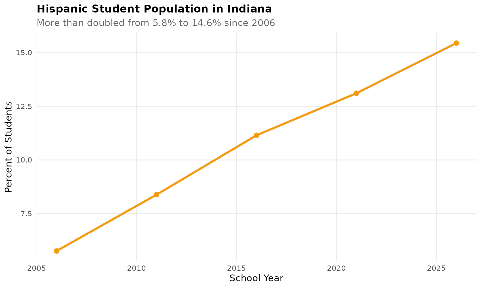
5. COVID erased 5,600 kindergartners in one year
Indiana kindergarten enrollment dropped from 78,649 in 2020 to 72,993 in 2021 – a loss of nearly 5,700 students. Recovery has been uneven.
k_trend <- enr %>%
  filter(is_state, subgroup == "total_enrollment",
         grade_level %in% c("K", "01", "06", "12")) %>%
  mutate(grade_label = case_when(
    grade_level == "K" ~ "Kindergarten",
    grade_level == "01" ~ "Grade 1",
    grade_level == "06" ~ "Grade 6",
    grade_level == "12" ~ "Grade 12"
  ))

stopifnot(nrow(k_trend) > 0)

k_trend %>%
  filter(grade_level == "K") %>%
  select(end_year, n_students)
#>    end_year n_students
#> 1      2017      76870
#> 2      2018      77905
#> 3      2019      75746
#> 4      2020      78649
#> 5      2021      72993
#> 6      2022      76514
#> 7      2023      74124
#> 8      2024      72955
#> 9      2025      71379
#> 10     2026      69849

ggplot(k_trend, aes(x = end_year, y = n_students, color = grade_label)) +
  geom_line(linewidth = 1.2) +
  geom_point(size = 2.5) +
  geom_vline(xintercept = 2021, linetype = "dashed", color = "red", alpha = 0.5) +
  scale_y_continuous(labels = comma) +
  labs(title = "COVID Hit Indiana Kindergarten Hard",
       subtitle = "Lost 5,600 kindergartners between 2020 and 2021",
       x = "School Year", y = "Students", color = "") +
  theme_readme()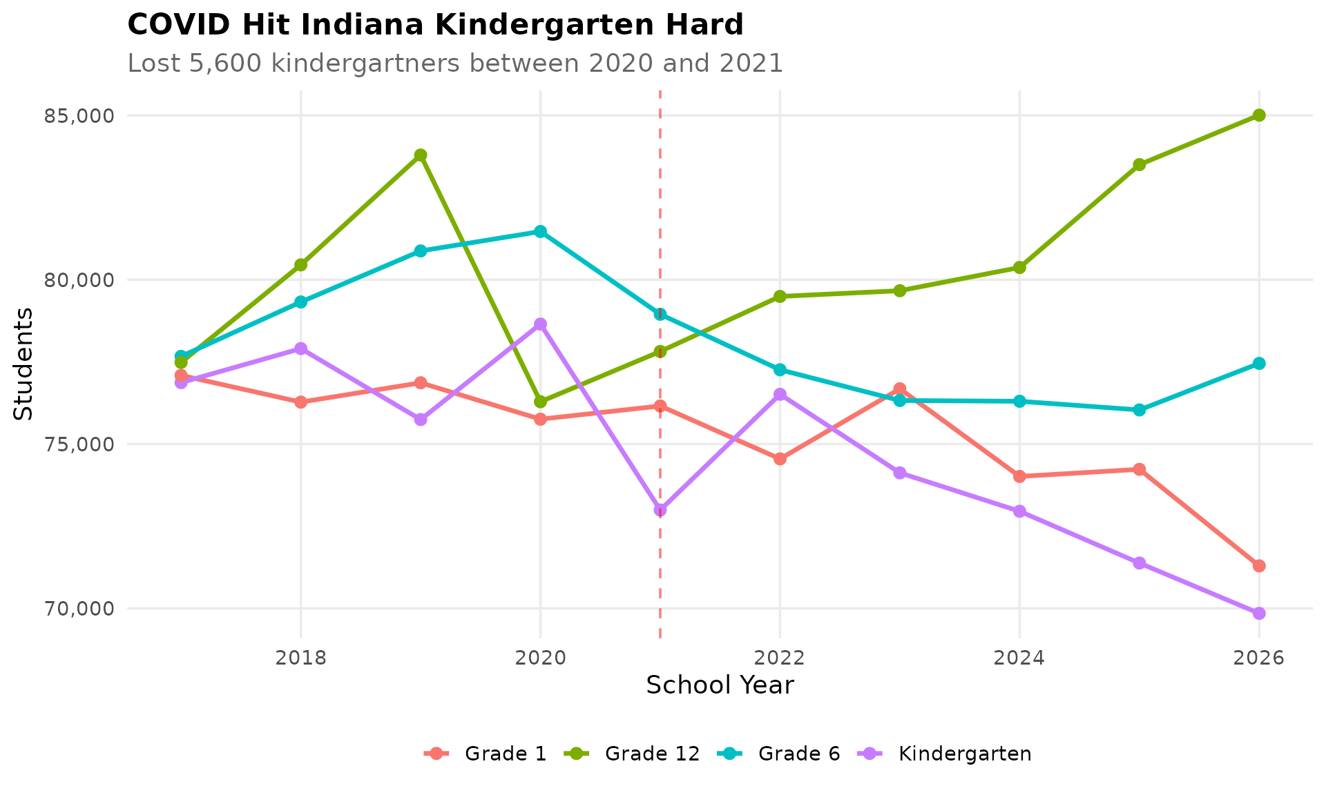
6. White enrollment dropped 15 points while Hispanic surged
Indiana’s racial composition shifted dramatically since 2006. White students went from 78% to 63% while Hispanic students rose from 6% to 15%. Black enrollment has been comparatively stable.
race_trend <- enr_long %>%
  filter(is_state, grade_level == "TOTAL", subgroup %in% c("black", "hispanic", "white")) %>%
  mutate(subgroup = factor(subgroup, levels = c("white", "black", "hispanic"),
                           labels = c("White", "Black", "Hispanic")))

stopifnot(nrow(race_trend) > 0)

race_trend %>%
  select(end_year, subgroup, pct) %>%
  mutate(pct = round(pct * 100, 1))
#>    end_year subgroup  pct
#> 1      2006    White 78.0
#> 2      2006    Black 11.5
#> 3      2006 Hispanic  5.8
#> 4      2011    White 73.1
#> 5      2011    Black 12.1
#> 6      2011 Hispanic  8.4
#> 7      2016    White 69.3
#> 8      2016    Black 12.4
#> 9      2016 Hispanic 11.1
#> 10     2021    White 65.8
#> 11     2021    Black 12.9
#> 12     2021 Hispanic 13.1
#> 13     2026    White 61.4
#> 14     2026    Black 13.9
#> 15     2026 Hispanic 15.4

ggplot(race_trend, aes(x = end_year, y = pct * 100, color = subgroup)) +
  geom_line(linewidth = 1.2) +
  geom_point(size = 2.5) +
  scale_color_manual(values = c("White" = colors["white"], "Black" = colors["black"],
                                "Hispanic" = colors["hispanic"])) +
  labs(title = "Indiana's Racial Demographics Are Shifting Fast",
       subtitle = "White share fell 15 points while Hispanic share nearly tripled",
       x = "School Year", y = "Percent of Students", color = "") +
  theme_readme()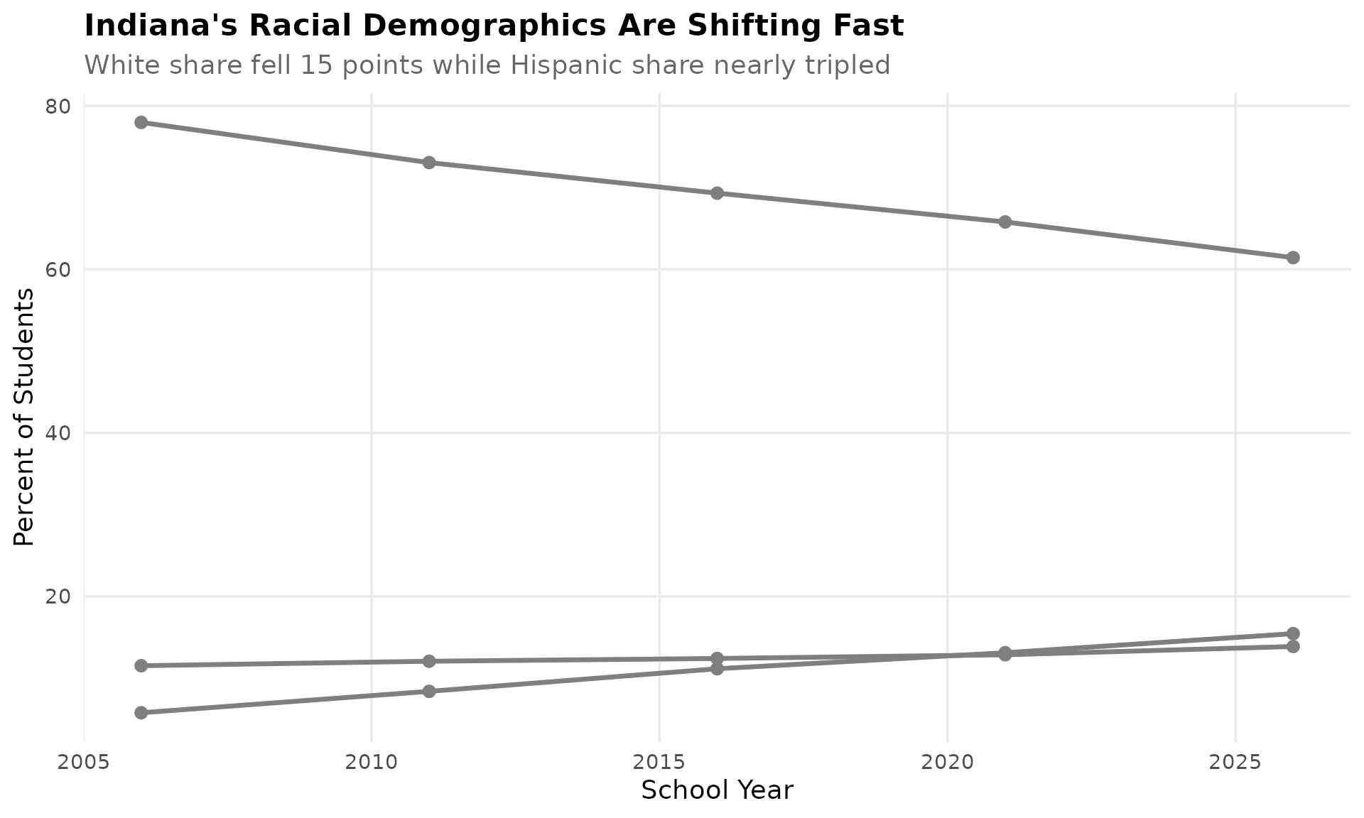
7. Gary lost 73% of its students since 2006
Gary Community School Corp went from 15,119 students in 2006 to just 4,025 in 2024, one of the steepest enrollment declines of any school district in America.
gary <- enr_long %>%
  filter(is_corporation, grepl("Gary Community", corporation_name, ignore.case = TRUE),
         subgroup == "total_enrollment", grade_level == "TOTAL")

stopifnot(nrow(gary) > 0)

gary %>% select(end_year, corporation_name, n_students)
#>   end_year           corporation_name n_students
#> 1     2006 Gary Community School Corp      15119
#> 2     2011 Gary Community School Corp      11161
#> 3     2016 Gary Community School Corp       6480
#> 4     2021 Gary Community School Corp       4770
#> 5     2026 Gary Community School Corp       4025

ggplot(gary, aes(x = end_year, y = n_students)) +
  geom_line(linewidth = 1.5, color = colors["total"]) +
  geom_point(size = 3, color = colors["total"]) +
  scale_y_continuous(labels = comma, limits = c(0, NA)) +
  labs(title = "Gary Community Schools Collapse",
       subtitle = "From 15,100 to 4,000 -- a 73% decline since 2006",
       x = "School Year", y = "Students") +
  theme_readme()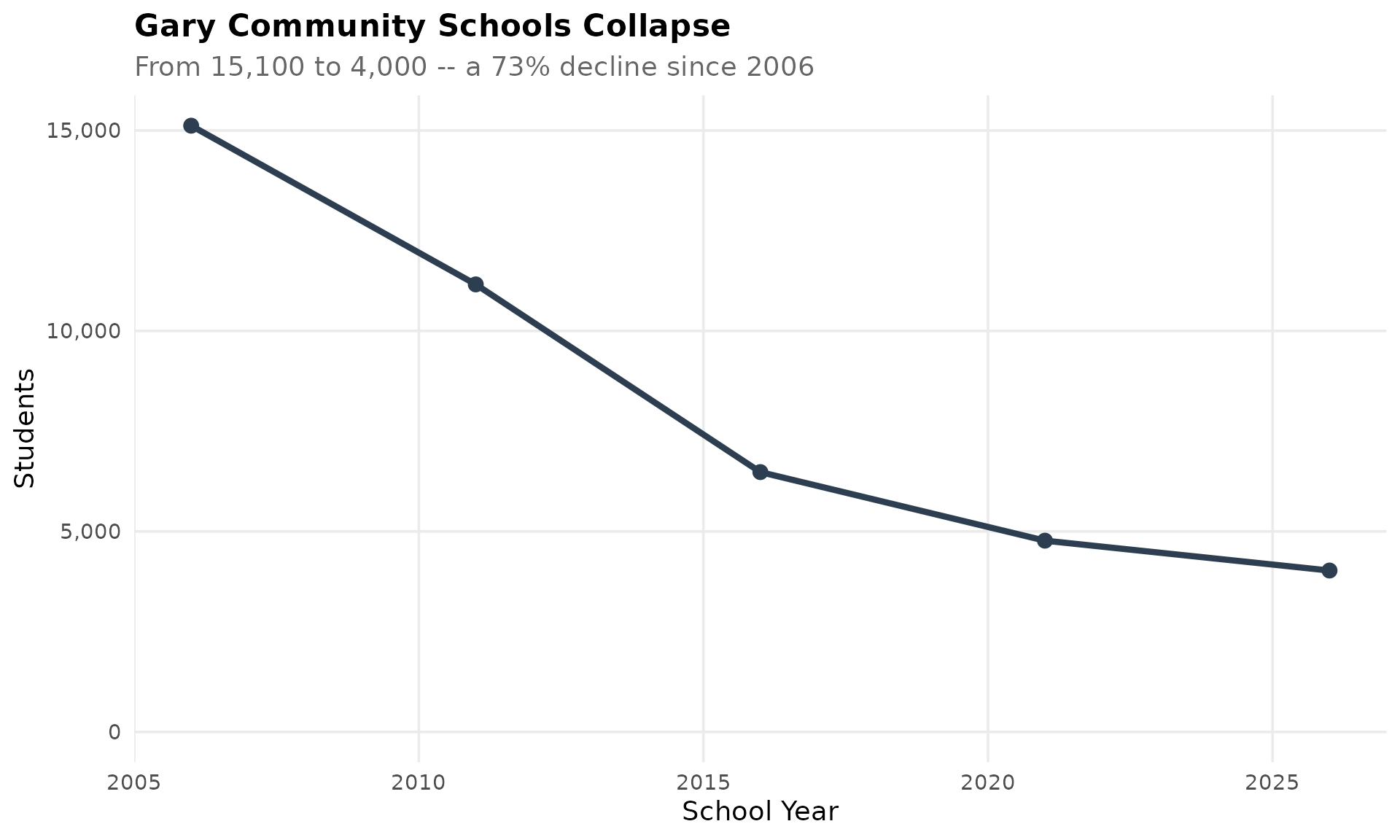
8. Indiana Connections Academy is the largest virtual school
Indiana Connections Academy serves over 5,400 students, making it by far the largest virtual school in the state.
virtual <- enr_current %>%
  filter(grepl("Virtual|Online|Connections|Digital", corporation_name, ignore.case = TRUE),
         grade_level == "TOTAL", subgroup == "total_enrollment") %>%
  distinct(corporation_name, .keep_all = TRUE) %>%
  arrange(desc(n_students)) %>%
  head(10) %>%
  mutate(corp_label = reorder(corporation_name, n_students))

stopifnot(nrow(virtual) > 0)

virtual %>% select(corporation_name, n_students)
#>                    corporation_name n_students
#> 1  Indiana Connections Academy 7-12       5027
#> 2   Indiana Connections Academy K-6       1631
#> 3 Phalen Virtual Leadership Academy        255
#> 4          Paramount Online Academy        151

ggplot(virtual, aes(x = corp_label, y = n_students)) +
  geom_col(fill = colors["total"]) +
  coord_flip() +
  scale_y_continuous(labels = comma) +
  labs(title = "Indiana's Virtual Schools",
       subtitle = "Indiana Connections Academy leads with 5,400+ students",
       x = "", y = "Students") +
  theme_readme()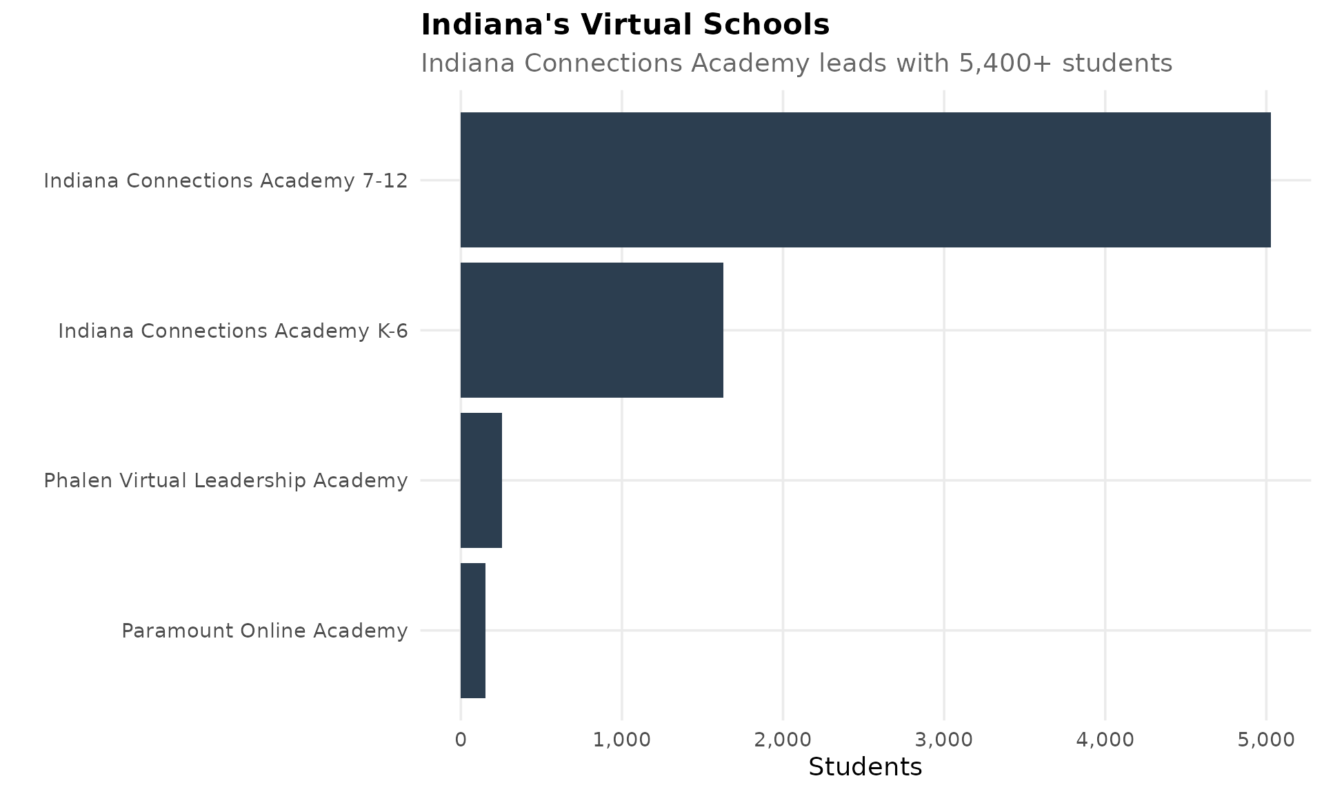
9. Evansville is slowly losing students
Evansville Vanderburgh School Corp peaked around 22,800 and has gradually declined to about 21,400 – a modest but steady loss of about 5% over the past decade.
evansville <- enr %>%
  filter(is_corporation, grepl("Evansville Vanderburgh", corporation_name, ignore.case = TRUE),
         subgroup == "total_enrollment", grade_level == "TOTAL")

stopifnot(nrow(evansville) > 0)

evansville %>% select(end_year, corporation_name, n_students)
#>    end_year                   corporation_name n_students
#> 1      2017 Evansville Vanderburgh School Corp      22801
#> 2      2018 Evansville Vanderburgh School Corp      22844
#> 3      2019 Evansville Vanderburgh School Corp      22601
#> 4      2020 Evansville Vanderburgh School Corp      22822
#> 5      2021 Evansville Vanderburgh School Corp      22192
#> 6      2022 Evansville Vanderburgh School Corp      21942
#> 7      2023 Evansville Vanderburgh School Corp      21741
#> 8      2024 Evansville Vanderburgh School Corp      21442
#> 9      2025 Evansville Vanderburgh School Corp      21589
#> 10     2026 Evansville Vanderburgh School Corp      20914

ggplot(evansville, aes(x = end_year, y = n_students)) +
  geom_line(linewidth = 1.5, color = colors["total"]) +
  geom_point(size = 3, color = colors["total"]) +
  scale_y_continuous(labels = comma, limits = c(0, NA)) +
  labs(title = "Evansville Vanderburgh School Corp",
       subtitle = "Gradual decline from 22,800 to 21,400 over the past decade",
       x = "School Year", y = "Students") +
  theme_readme()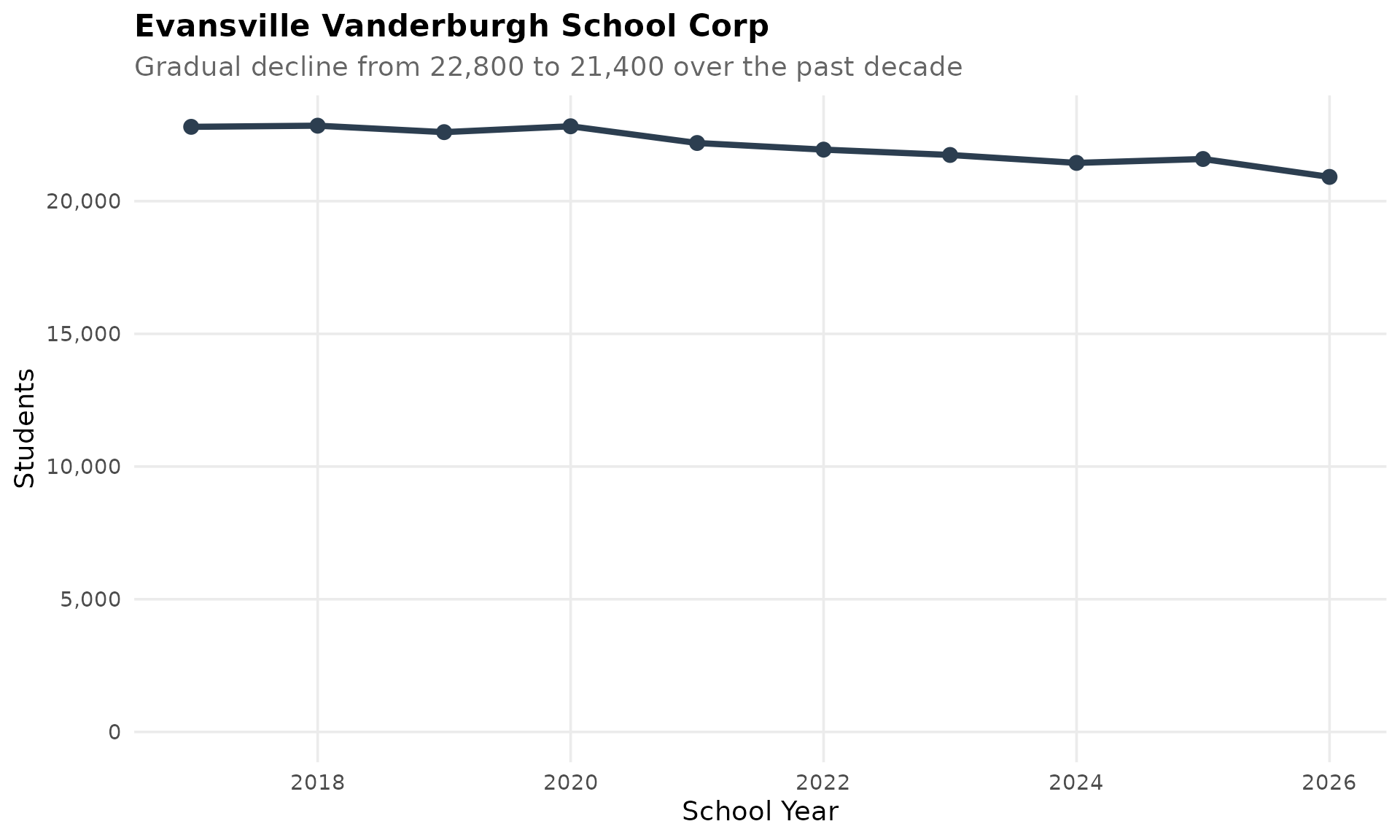
10. Indiana’s school system has grown more fragmented
Indiana went from 330 corporations in 2006 to 418 in 2024. Rather than consolidating, the state has added charter schools and virtual academies that count as new corporations.
corp_counts <- enr_long %>%
  filter(is_corporation, subgroup == "total_enrollment", grade_level == "TOTAL") %>%
  group_by(end_year) %>%
  summarize(n_corporations = n(), .groups = "drop")

stopifnot(nrow(corp_counts) > 0)

corp_counts
#> # A tibble: 5 × 2
#>   end_year n_corporations
#>      <dbl>          <int>
#> 1     2006            330
#> 2     2011            357
#> 3     2016            386
#> 4     2021            406
#> 5     2026            430

ggplot(corp_counts, aes(x = end_year, y = n_corporations)) +
  geom_line(linewidth = 1.5, color = colors["total"]) +
  geom_point(size = 3, color = colors["total"]) +
  labs(title = "Indiana's Corporation Count Has Grown",
       subtitle = "From 330 in 2006 to 418 in 2024 -- charters and virtual schools drive the increase",
       x = "School Year", y = "Number of Corporations") +
  theme_readme()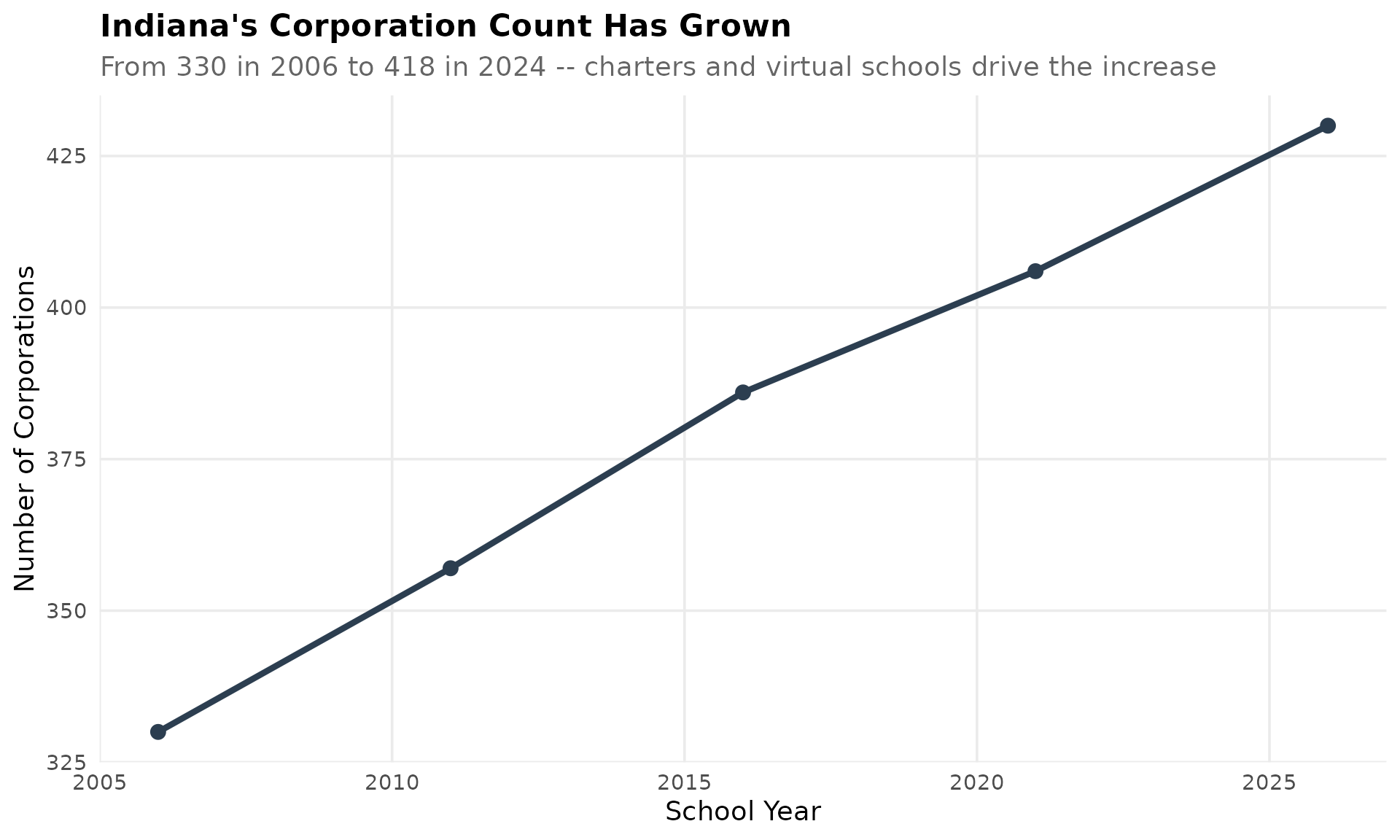
11. Fort Wayne is Indiana’s largest district at 28,500 students
Fort Wayne Community Schools is the largest district in Indiana with about 28,500 students, edging out Indianapolis Public Schools which has fallen to around 21,900.
fort_wayne <- enr %>%
  filter(is_corporation, grepl("Fort Wayne Community", corporation_name, ignore.case = TRUE),
         subgroup == "total_enrollment", grade_level == "TOTAL")

stopifnot(nrow(fort_wayne) > 0)

fort_wayne %>% select(end_year, corporation_name, n_students)
#>    end_year             corporation_name n_students
#> 1      2017 Fort Wayne Community Schools      29377
#> 2      2018 Fort Wayne Community Schools      29469
#> 3      2019 Fort Wayne Community Schools      29404
#> 4      2020 Fort Wayne Community Schools      29486
#> 5      2021 Fort Wayne Community Schools      28460
#> 6      2022 Fort Wayne Community Schools      28778
#> 7      2023 Fort Wayne Community Schools      28613
#> 8      2024 Fort Wayne Community Schools      28504
#> 9      2025 Fort Wayne Community Schools      28549
#> 10     2026 Fort Wayne Community Schools      28200

ggplot(fort_wayne, aes(x = end_year, y = n_students)) +
  geom_line(linewidth = 1.5, color = colors["total"]) +
  geom_point(size = 3, color = colors["total"]) +
  scale_y_continuous(labels = comma, limits = c(0, NA)) +
  labs(title = "Fort Wayne Community Schools",
       subtitle = "Indiana's largest district at ~28,500 students",
       x = "School Year", y = "Students") +
  theme_readme()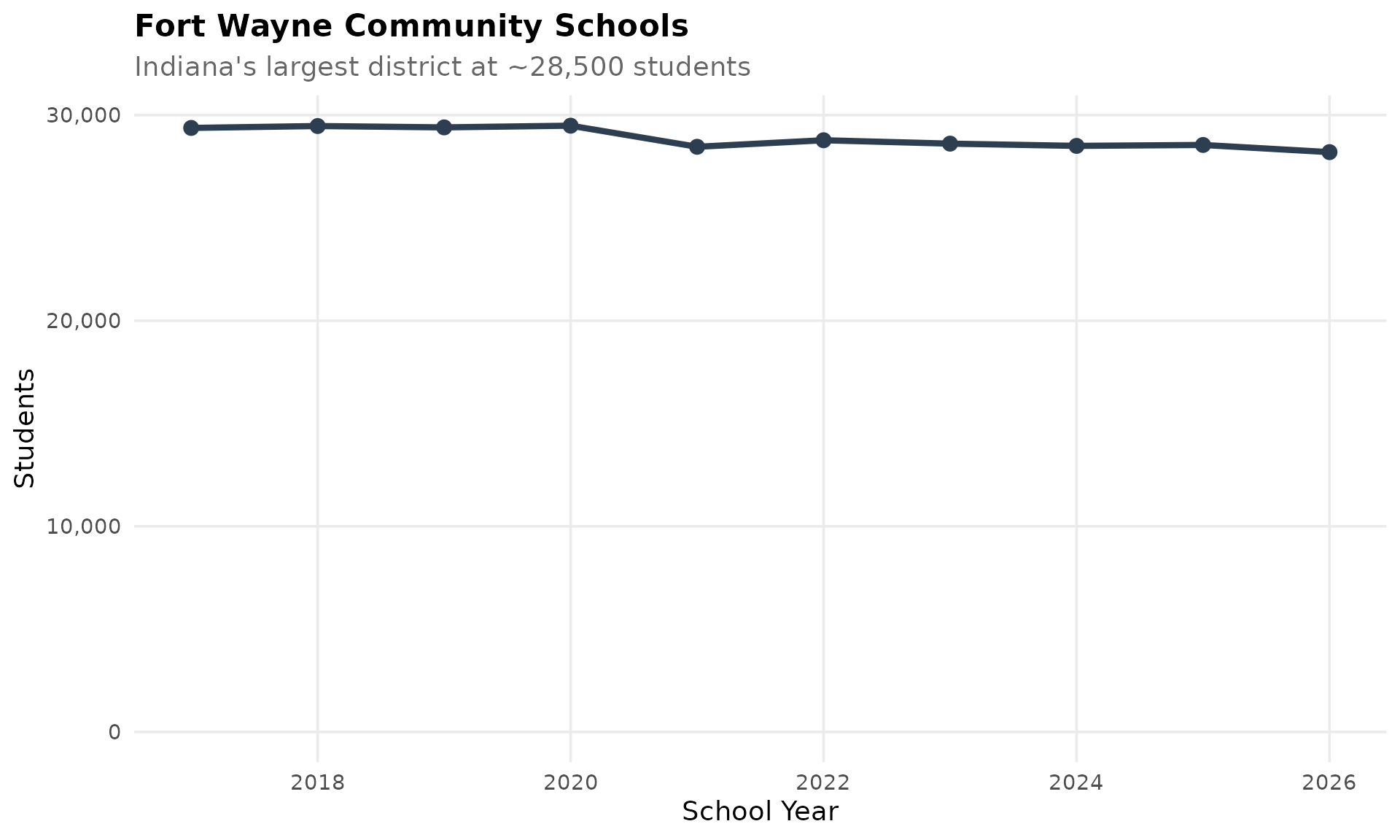
12. Black enrollment share has risen slightly since 2006
Despite a common misconception, Indiana’s Black student share has actually edged up from 11.5% in 2006 to 13.4% in 2024, while Black student counts grew from 125,000 to 138,000.
black_trend <- enr_long %>%
  filter(is_state, grade_level == "TOTAL", subgroup == "black")

stopifnot(nrow(black_trend) > 0)

black_trend %>% select(end_year, n_students, pct) %>%
  mutate(pct_display = round(pct * 100, 1))
#>   end_year n_students       pct pct_display
#> 1     2006     125305 0.1151895        11.5
#> 2     2011     126350 0.1206699        12.1
#> 3     2016     129809 0.1240379        12.4
#> 4     2021     132917 0.1285737        12.9
#> 5     2026     142645 0.1386969        13.9

ggplot(black_trend, aes(x = end_year, y = pct * 100)) +
  geom_line(linewidth = 1.5, color = colors["black"]) +
  geom_point(size = 3, color = colors["black"]) +
  labs(title = "Black Student Enrollment Share in Indiana",
       subtitle = "Edged up from 11.5% to 13.4% since 2006",
       x = "School Year", y = "Percent of Students") +
  theme_readme()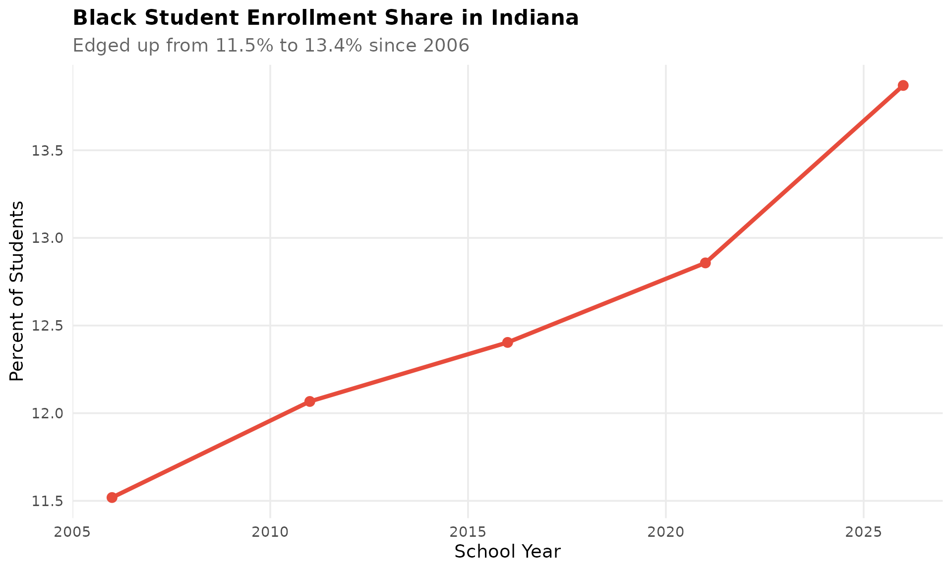
13. South Bend has lost a third of its students
South Bend Community School Corp went from nearly 21,900 students in 2006 to about 14,500 in 2024 – a loss of 34%.
south_bend <- enr_long %>%
  filter(is_corporation, grepl("South Bend Community", corporation_name, ignore.case = TRUE),
         subgroup == "total_enrollment", grade_level == "TOTAL")

stopifnot(nrow(south_bend) > 0)

south_bend %>% select(end_year, corporation_name, n_students)
#>   end_year                 corporation_name n_students
#> 1     2006    South Bend Community Sch Corp      21861
#> 2     2011    South Bend Community Sch Corp      19948
#> 3     2016    South Bend Community Sch Corp      18680
#> 4     2021 South Bend Community School Corp      16302
#> 5     2026 South Bend Community School Corp      12851

ggplot(south_bend, aes(x = end_year, y = n_students)) +
  geom_line(linewidth = 1.5, color = colors["total"]) +
  geom_point(size = 3, color = colors["total"]) +
  scale_y_continuous(labels = comma, limits = c(0, NA)) +
  labs(title = "South Bend Community Schools",
       subtitle = "Lost 34% of enrollment since 2006",
       x = "School Year", y = "Students") +
  theme_readme()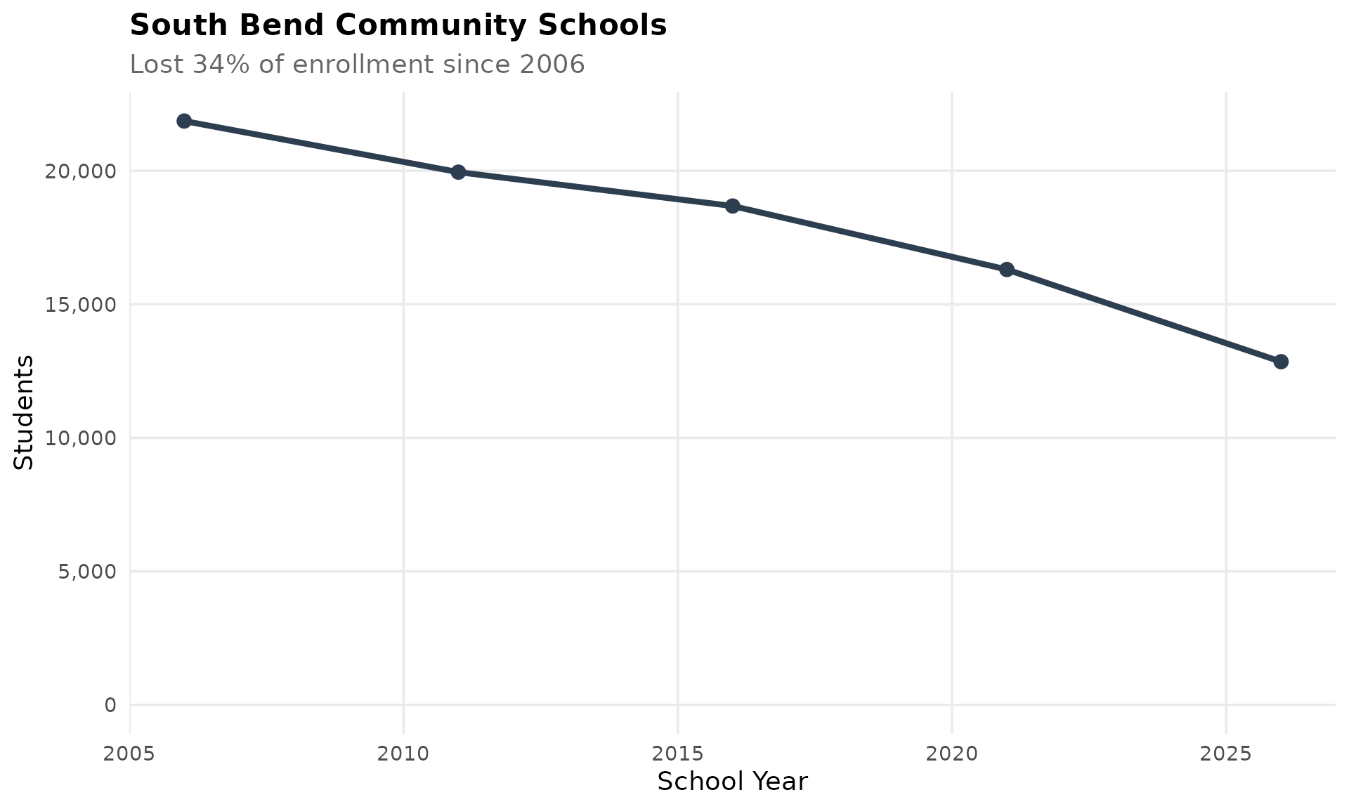
14. Asian students are the fastest-growing demographic in percentage terms
Asian enrollment went from 1.2% to 3.0% of Indiana’s total since 2006. While a smaller population than Hispanic growth, it represents a 2.5x increase in share.
asian_trend <- enr_long %>%
  filter(is_state, grade_level == "TOTAL", subgroup == "asian")

stopifnot(nrow(asian_trend) > 0)

asian_trend %>% select(end_year, n_students, pct) %>%
  mutate(pct_display = round(pct * 100, 1))
#>   end_year n_students        pct pct_display
#> 1     2006          0 0.00000000         0.0
#> 2     2011      16970 0.01620711         1.6
#> 3     2016      22519 0.02151784         2.2
#> 4     2021      28265 0.02734138         2.7
#> 5     2026      33483 0.03255625         3.3

ggplot(asian_trend, aes(x = end_year, y = pct * 100)) +
  geom_line(linewidth = 1.5, color = colors["asian"]) +
  geom_point(size = 3, color = colors["asian"]) +
  labs(title = "Asian Student Enrollment in Indiana",
       subtitle = "Share grew from 1.2% to 3.0% since 2006",
       x = "School Year", y = "Percent of Students") +
  theme_readme()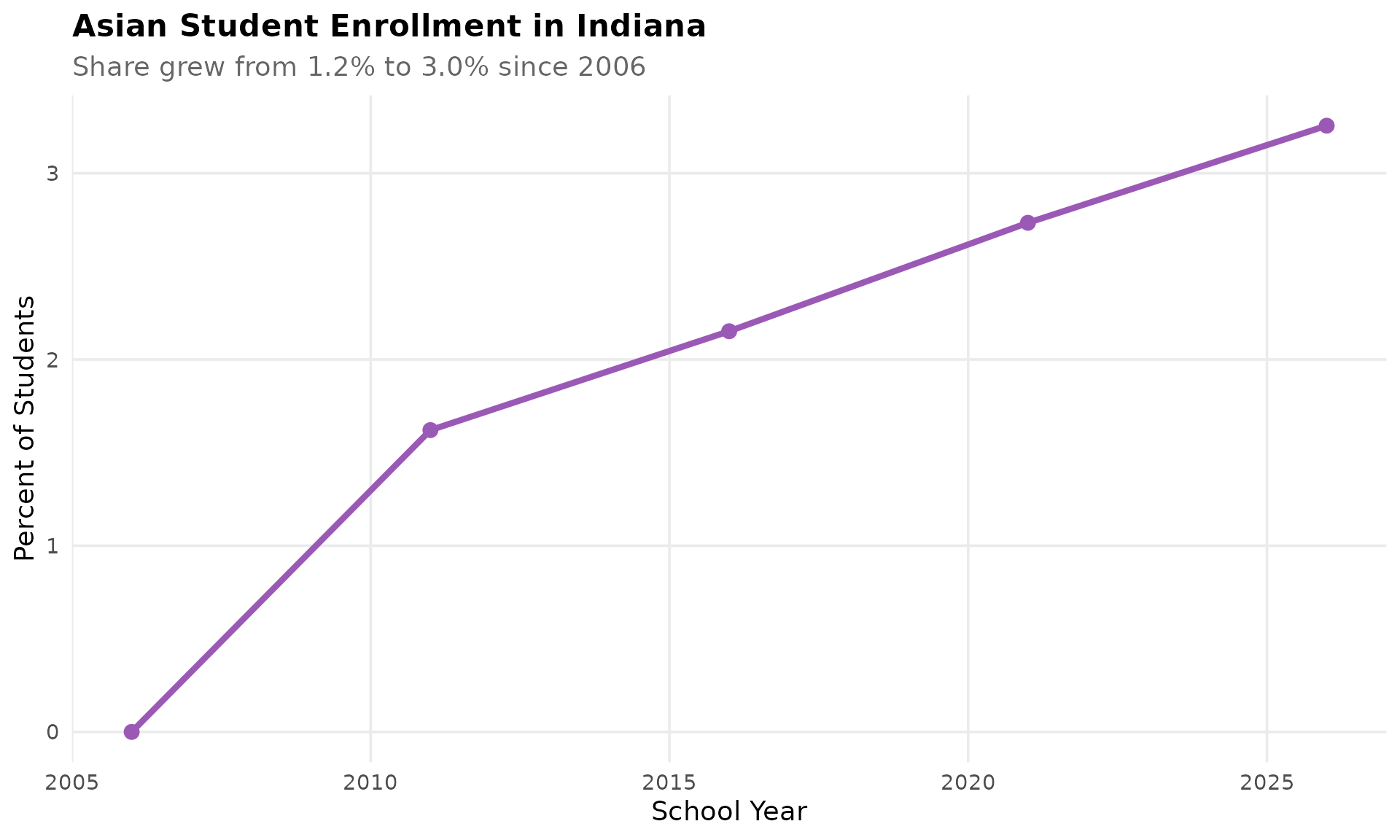
15. The top 20 corporations serve 29% of all students
The 20 largest corporations educate nearly 300,000 of Indiana’s 1.03 million students. Fort Wayne, Indianapolis, and Evansville lead the pack.
top_corps <- enr_current %>%
  filter(is_corporation, grade_level == "TOTAL", subgroup == "total_enrollment") %>%
  arrange(desc(n_students)) %>%
  head(20) %>%
  mutate(corp_label = reorder(corporation_name, n_students))

stopifnot(nrow(top_corps) > 0)

top_corps %>% select(corporation_name, n_students)
#>                      corporation_name n_students
#> 1        Fort Wayne Community Schools      28200
#> 2  Evansville Vanderburgh School Corp      20914
#> 3       Hamilton Southeastern Schools      20633
#> 4         Indianapolis Public Schools      19774
#> 5               MSD Lawrence Township      16709
#> 6                 Carmel Clay Schools      15913
#> 7                  MSD Wayne Township      15734
#> 8              Perry Township Schools      15726
#> 9              Tippecanoe School Corp      13423
#> 10            Vigo County School Corp      12986
#> 11   South Bend Community School Corp      12851
#> 12     Franklin Township Com Sch Corp      11572
#> 13                MSD Warren Township      11502
#> 14        Bartholomew Con School Corp      11459
#> 15            MSD Washington Township      11325
#> 16        New Albany-Floyd Co Con Sch      11218
#> 17    Penn-Harris-Madison School Corp      11185
#> 18         Avon Community School Corp      10735
#> 19                  MSD Pike Township      10640
#> 20       Greater Clark County Schools      10627

ggplot(top_corps, aes(x = corp_label, y = n_students)) +
  geom_col(fill = colors["total"]) +
  coord_flip() +
  scale_y_continuous(labels = comma) +
  labs(title = "Top 20 Corporations by Enrollment",
       subtitle = "The largest 20 districts serve 29% of Indiana students",
       x = "", y = "Students") +
  theme_readme()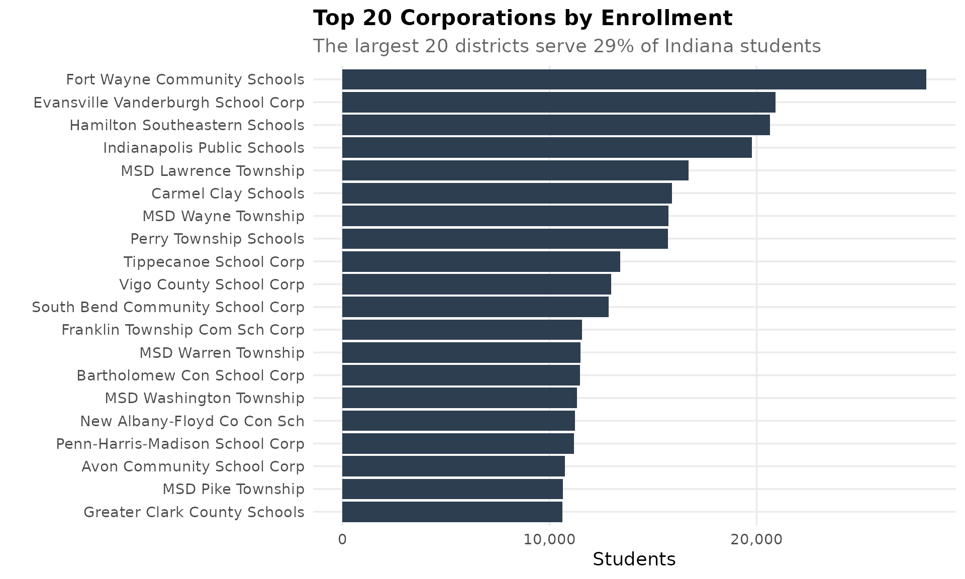
Session Info
sessionInfo()
#> R version 4.5.2 (2025-10-31)
#> Platform: x86_64-pc-linux-gnu
#> Running under: Ubuntu 24.04.3 LTS
#>
#> Matrix products: default
#> BLAS:   /usr/lib/x86_64-linux-gnu/openblas-pthread/libblas.so.3
#> LAPACK: /usr/lib/x86_64-linux-gnu/openblas-pthread/libopenblasp-r0.3.26.so;  LAPACK version 3.12.0
#>
#> locale:
#>  [1] LC_CTYPE=C.UTF-8       LC_NUMERIC=C           LC_TIME=C.UTF-8
#>  [4] LC_COLLATE=C.UTF-8     LC_MONETARY=C.UTF-8    LC_MESSAGES=C.UTF-8
#>  [7] LC_PAPER=C.UTF-8       LC_NAME=C              LC_ADDRESS=C
#> [10] LC_TELEPHONE=C         LC_MEASUREMENT=C.UTF-8 LC_IDENTIFICATION=C
#>
#> time zone: UTC
#> tzcode source: system (glibc)
#>
#> attached base packages:
#> [1] stats     graphics  grDevices utils     datasets  methods   base
#>
#> other attached packages:
#> [1] scales_1.4.0       dplyr_1.2.0        ggplot2_4.0.2      inschooldata_0.2.0
#>
#> loaded via a namespace (and not attached):
#>  [1] gtable_0.3.6       jsonlite_2.0.0     compiler_4.5.2     tidyselect_1.2.1
#>  [5] jquerylib_0.1.4    systemfonts_1.3.2  textshaping_1.0.5  readxl_1.4.5
#>  [9] yaml_2.3.12        fastmap_1.2.0      R6_2.6.1           labeling_0.4.3
#> [13] generics_0.1.4     curl_7.0.0         knitr_1.51         tibble_3.3.1
#> [17] desc_1.4.3         bslib_0.10.0       pillar_1.11.1      RColorBrewer_1.1-3
#> [21] rlang_1.1.7        cachem_1.1.0       xfun_0.56          fs_1.6.7
#> [25] sass_0.4.10        S7_0.2.1           cli_3.6.5          pkgdown_2.2.0
#> [29] withr_3.0.2        magrittr_2.0.4     digest_0.6.39      grid_4.5.2
#> [33] rappdirs_0.3.4     lifecycle_1.0.5    vctrs_0.7.1        evaluate_1.0.5
#> [37] glue_1.8.0         cellranger_1.1.0   farver_2.1.2       codetools_0.2-20
#> [41] ragg_1.5.1         rmarkdown_2.30     purrr_1.2.1        httr_1.4.8
#> [45] tools_4.5.2        pkgconfig_2.0.3    htmltools_0.5.9