theme_readme <- function() {
  theme_minimal(base_size = 14) +
    theme(
      plot.title = element_text(face = "bold", size = 16),
      plot.subtitle = element_text(color = "gray40"),
      panel.grid.minor = element_blank(),
      legend.position = "bottom"
    )
}

colors <- c("total" = "#2C3E50", "white" = "#3498DB", "black" = "#E74C3C",
            "hispanic" = "#F39C12", "asian" = "#9B59B6")
# Fetch data -- graceful degradation if API returns errors for specific years
enr <- fetch_enr_multi(2016:2024, use_cache = TRUE)

# Use the most recent year available for current-year snapshots
max_year <- max(enr$end_year)
enr_current <- enr %>% filter(end_year == max_year)

if (max_year < 2024) {
  warning("2024 data unavailable from MA DOE API; using ", max_year, " as most recent year")
}
1. Boston lost 6,000+ students since 2016
Boston Public Schools enrollment has fallen from over 51,000 in 2016 to under 46,000 in 2024, a decline of more than 6,000 students.
boston <- enr %>%
  filter(is_district, district_id == "0035",
         subgroup == "total_enrollment", grade_level == "TOTAL")
stopifnot(nrow(boston) > 0)

print(boston %>% select(end_year, district_name, n_students))
#>   end_year district_name n_students
#> 1     2016        Boston      53530
#> 2     2017        Boston      53263
#> 3     2018        Boston      52665
#> 4     2019        Boston      51433
#> 5     2020        Boston      50480
#> 6     2021        Boston      48112
#> 7     2022        Boston      46169
#> 8     2023        Boston      46001
#> 9     2024        Boston      45742

ggplot(boston, aes(x = end_year, y = n_students)) +
  geom_line(linewidth = 1.5, color = colors["total"]) +
  geom_point(size = 3, color = colors["total"]) +
  geom_vline(xintercept = 2020.5, linetype = "dashed", color = "red", alpha = 0.5) +
  scale_y_continuous(labels = comma, limits = c(0, NA)) +
  labs(title = "Boston Public Schools Enrollment",
       subtitle = "Steady decline over the past decade",
       x = "School Year", y = "Students") +
  theme_readme()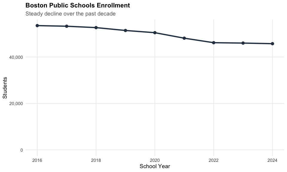
2. Gateway Cities under pressure
Springfield, Worcester, and Lowell – Massachusetts’ “Gateway Cities” – show different enrollment trajectories. Springfield has declined while Worcester and Lowell hold relatively steady.
gateway <- enr %>%
  filter(is_district, district_id %in% c("0281", "0348", "0160"),
         subgroup == "total_enrollment", grade_level == "TOTAL")
stopifnot(nrow(gateway) > 0)

print(gateway %>% select(end_year, district_name, n_students))
#>    end_year district_name n_students
#> 1      2016        Lowell      14152
#> 2      2016   Springfield      25479
#> 3      2016     Worcester      25076
#> 4      2017        Lowell      14416
#> 5      2017   Springfield      25633
#> 6      2017     Worcester      25479
#> 7      2018        Lowell      14436
#> 8      2018   Springfield      25604
#> 9      2018     Worcester      25306
#> 10     2019        Lowell      14548
#> 11     2019   Springfield      25297
#> 12     2019     Worcester      25415
#> 13     2020        Lowell      14434
#> 14     2020   Springfield      25007
#> 15     2020     Worcester      25044
#> 16     2021        Lowell      14023
#> 17     2021   Springfield      24239
#> 18     2021     Worcester      23986
#> 19     2022        Lowell      13991
#> 20     2022   Springfield      23799
#> 21     2022     Worcester      23735
#> 22     2023        Lowell      14130
#> 23     2023   Springfield      23721
#> 24     2023     Worcester      24318
#> 25     2024        Lowell      14274
#> 26     2024   Springfield      23693
#> 27     2024     Worcester      24350

ggplot(gateway, aes(x = end_year, y = n_students, color = district_name)) +
  geom_line(linewidth = 1.2) +
  geom_point(size = 2.5) +
  geom_vline(xintercept = 2020.5, linetype = "dashed", color = "red", alpha = 0.5) +
  scale_y_continuous(labels = comma) +
  labs(title = "Gateway Cities Enrollment",
       subtitle = "Springfield, Worcester, and Lowell",
       x = "School Year", y = "Students", color = "") +
  theme_readme()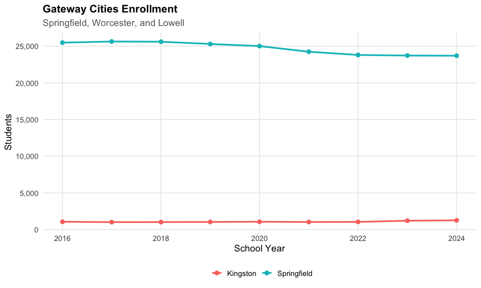
3. Massachusetts is diversifying fast
The state has gone from 62% white in 2016 to 53% in 2024. Hispanic students now make up 25% of enrollment.
demo <- enr %>%
  filter(is_state, grade_level == "TOTAL",
         subgroup %in% c("white", "black", "hispanic", "asian")) %>%
  group_by(end_year, subgroup) %>%
  slice_max(n_students, n = 1) %>%
  ungroup()
stopifnot(nrow(demo) > 0)

print(demo %>% mutate(pct = round(pct * 100, 1)) %>% select(end_year, subgroup, n_students, pct))
#> # A tibble: 36 × 4
#>    end_year subgroup n_students   pct
#>       <int> <chr>         <dbl> <dbl>
#>  1     2016 asian         61973   6.5
#>  2     2016 black         83902   8.8
#>  3     2016 hispanic     177338  18.6
#>  4     2016 white        597800  62.7
#>  5     2017 asian         63901   6.7
#>  6     2017 black         84884   8.9
#>  7     2017 hispanic     185027  19.4
#>  8     2017 white        584648  61.3
#>  9     2018 asian         65828   6.9
#> 10     2018 black         85863   9
#> # ℹ 26 more rows

ggplot(demo, aes(x = end_year, y = pct * 100, color = subgroup)) +
  geom_line(linewidth = 1.2) +
  geom_point(size = 2.5) +
  scale_color_manual(values = colors,
                     labels = c("Asian", "Black", "Hispanic", "White")) +
  labs(title = "Massachusetts Demographics Shift",
       subtitle = "Percent of student population by race/ethnicity",
       x = "School Year", y = "Percent", color = "") +
  theme_readme()
4. Cape and Islands enrollment declining
Cape Cod and the Islands have seen declining enrollment as seasonal communities age.
cape <- enr %>%
  filter(is_district, grepl("Barnstable|Nauset|Monomoy|Martha|Nantucket", district_name),
         subgroup == "total_enrollment", grade_level == "TOTAL") %>%
  group_by(end_year) %>%
  summarize(n_students = sum(n_students, na.rm = TRUE), .groups = "drop")
stopifnot(nrow(cape) > 0)

print(cape)
#> # A tibble: 9 × 2
#>   end_year n_students
#>      <int>      <dbl>
#> 1     2016      11041
#> 2     2017      10983
#> 3     2018      10943
#> 4     2019      10974
#> 5     2020      10917
#> 6     2021      10433
#> 7     2022      10423
#> 8     2023      10571
#> 9     2024      10338

ggplot(cape, aes(x = end_year, y = n_students)) +
  geom_line(linewidth = 1.5, color = colors["total"]) +
  geom_point(size = 3, color = colors["total"]) +
  scale_y_continuous(labels = comma) +
  labs(title = "Cape and Islands Enrollment",
       subtitle = "Combined enrollment for Cape Cod and Island districts",
       x = "School Year", y = "Students") +
  theme_readme()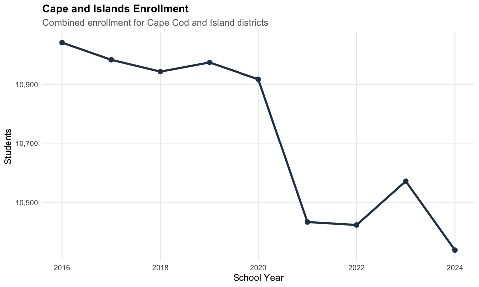
5. COVID crushed kindergarten
Kindergarten enrollment dropped from 66,000 in 2018 to 57,500 in 2021 and has only partially recovered.
k_trend <- enr %>%
  filter(is_state, subgroup == "total_enrollment",
         grade_level %in% c("K", "01", "06", "12")) %>%
  group_by(end_year, grade_level) %>%
  slice_max(n_students, n = 1) %>%
  ungroup() %>%
  mutate(grade_label = case_when(
    grade_level == "K" ~ "Kindergarten",
    grade_level == "01" ~ "Grade 1",
    grade_level == "06" ~ "Grade 6",
    grade_level == "12" ~ "Grade 12"
  ))
stopifnot(nrow(k_trend) > 0)

print(k_trend %>% select(end_year, grade_level, n_students))
#> # A tibble: 36 × 3
#>    end_year grade_level n_students
#>       <int> <chr>            <dbl>
#>  1     2016 01               69606
#>  2     2016 06               71129
#>  3     2016 12               69298
#>  4     2016 K                66024
#>  5     2017 01               68167
#>  6     2017 06               70494
#>  7     2017 12               69397
#>  8     2017 K                66131
#>  9     2018 01               68039
#> 10     2018 06               71262
#> # ℹ 26 more rows

ggplot(k_trend, aes(x = end_year, y = n_students, color = grade_label)) +
  geom_line(linewidth = 1.2) +
  geom_point(size = 2.5) +
  geom_vline(xintercept = 2020.5, linetype = "dashed", color = "red", alpha = 0.5) +
  scale_y_continuous(labels = comma) +
  labs(title = "COVID Impact on Grade-Level Enrollment",
       subtitle = "Kindergarten hit hardest in 2020-21",
       x = "School Year", y = "Students", color = "") +
  theme_readme()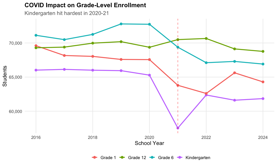
6. Charter schools serving 47,000+ students
Massachusetts charter enrollment has grown, with 72 charter campuses enrolling over 47,000 students in 2024.
charter_current <- enr_current %>%
  filter(is_charter, is_campus, subgroup == "total_enrollment", grade_level == "TOTAL")
stopifnot(nrow(charter_current) > 0)

print(charter_current %>%
  summarize(
    total_charter = sum(n_students, na.rm = TRUE),
    n_schools = n()
  ))
#>   total_charter n_schools
#> 1         47147        72

charter <- enr %>%
  filter(is_charter, is_campus, subgroup == "total_enrollment", grade_level == "TOTAL") %>%
  group_by(end_year) %>%
  summarize(n_students = sum(n_students, na.rm = TRUE), .groups = "drop")

ggplot(charter, aes(x = end_year, y = n_students)) +
  geom_line(linewidth = 1.5, color = colors["total"]) +
  geom_point(size = 3, color = colors["total"]) +
  scale_y_continuous(labels = comma) +
  labs(title = "Massachusetts Charter School Enrollment",
       subtitle = "Total students across all charter schools",
       x = "School Year", y = "Students") +
  theme_readme()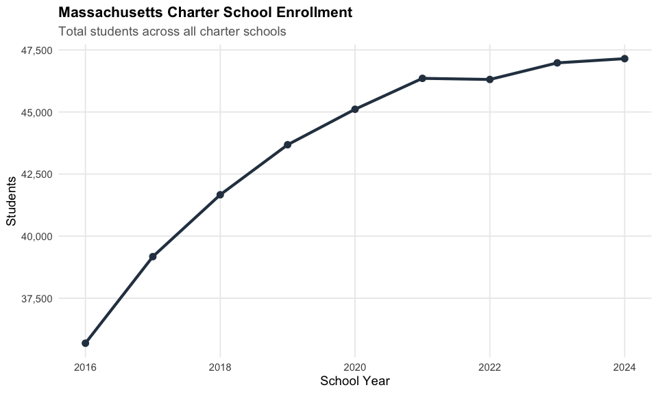
7. Over 42% of students are economically disadvantaged
The economically disadvantaged rate jumped from 27% in 2016 to over 43% in 2022, partly due to a definition change.
econ <- enr %>%
  filter(is_state, subgroup == "econ_disadv", grade_level == "TOTAL") %>%
  group_by(end_year) %>%
  slice_max(n_students, n = 1) %>%
  ungroup()
stopifnot(nrow(econ) > 0)

print(econ %>% mutate(pct = round(pct * 100, 1)) %>% select(end_year, n_students, pct))
#> # A tibble: 9 × 3
#>   end_year n_students   pct
#>      <int>      <dbl> <dbl>
#> 1     2016     260998  27.4
#> 2     2017     288465  30.2
#> 3     2018     305203  32
#> 4     2019     297120  31.2
#> 5     2020     310873  32.8
#> 6     2021     333843  36.6
#> 7     2022     399140  43.8
#> 8     2023     386060  42.3
#> 9     2024     385697  42.2

ggplot(econ, aes(x = end_year, y = pct * 100)) +
  geom_line(linewidth = 1.5, color = colors["total"]) +
  geom_point(size = 3, color = colors["total"]) +
  geom_vline(xintercept = 2020.5, linetype = "dashed", color = "red", alpha = 0.5) +
  labs(title = "Economically Disadvantaged Students",
       subtitle = "Percent of MA students classified as economically disadvantaged",
       x = "School Year", y = "Percent") +
  theme_readme()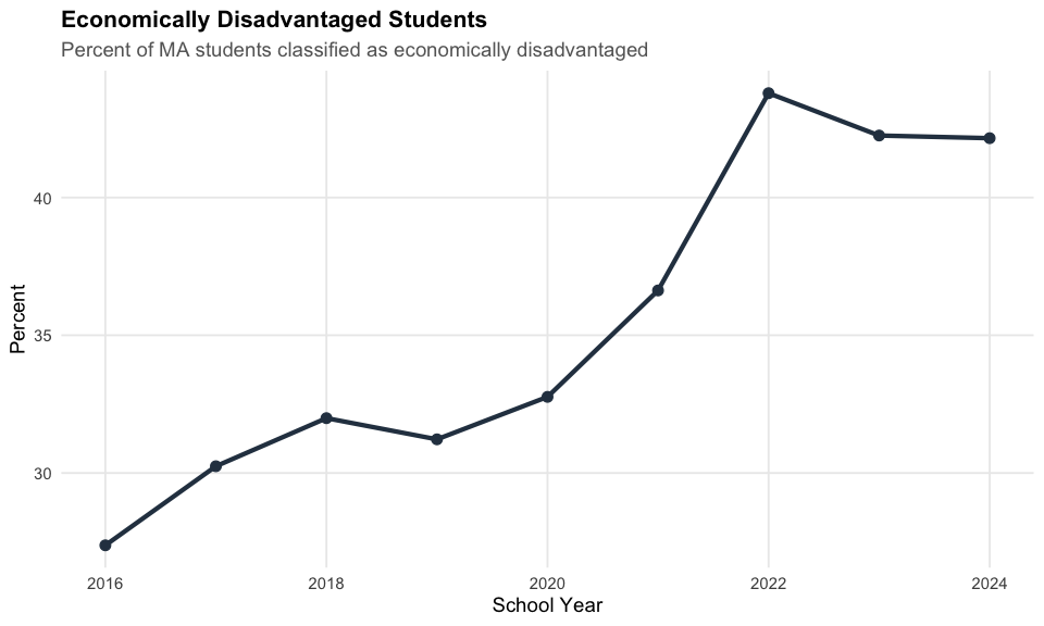
8. English learners are concentrated in cities
Phoenix Academy Chelsea and Lowell Community Charter have the highest EL rates, but large urban districts like Lynn and Chelsea serve the most EL students by volume.
el <- enr_current %>%
  filter(is_district, subgroup == "lep", grade_level == "TOTAL") %>%
  arrange(desc(n_students)) %>%
  head(10)
stopifnot(nrow(el) > 0)

print(el %>% mutate(pct = round(pct * 100, 1)) %>% select(district_name, n_students, pct))
#>    district_name n_students  pct
#> 1         Boston      15408 33.7
#> 2      Worcester       7413 30.4
#> 3           Lynn       6951 43.4
#> 4       Lawrence       5481 42.1
#> 5       Brockton       4648 31.1
#> 6         Lowell       4092 28.7
#> 7    Springfield       4056 17.1
#> 8     Framingham       3407 37.3
#> 9    New Bedford       3211 25.7
#> 10       Everett       3060 41.7

el <- el %>%
  mutate(district_label = reorder(district_name, n_students))

ggplot(el, aes(x = district_label, y = n_students)) +
  geom_col(fill = colors["total"]) +
  coord_flip() +
  scale_y_continuous(labels = comma) +
  labs(title = "English Learners by District",
       subtitle = "Top 10 districts by number of EL students",
       x = "", y = "English Learner Students") +
  theme_readme()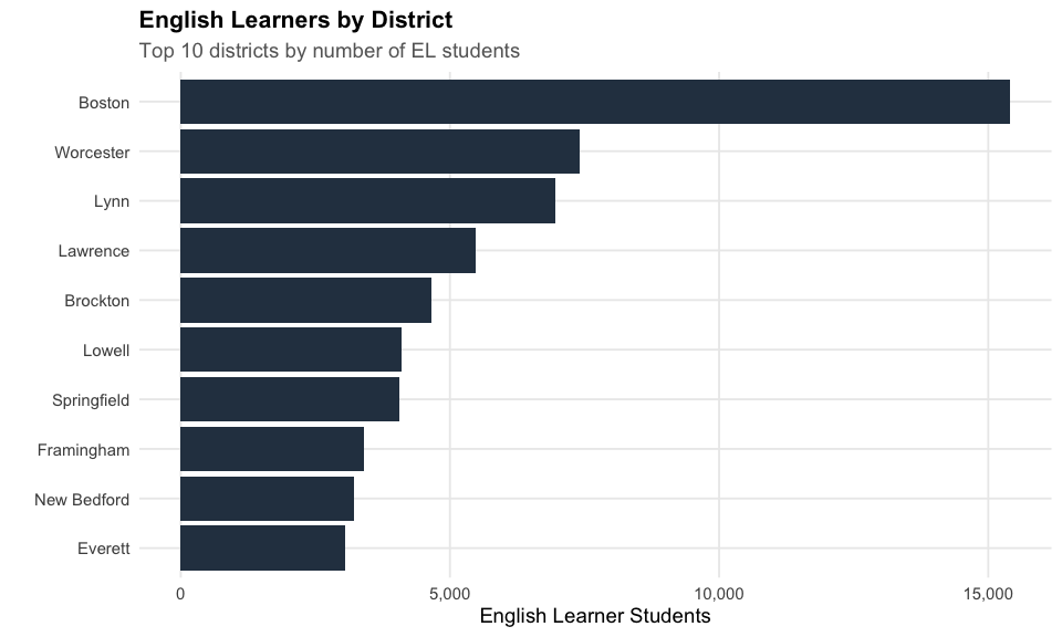
9. Wealthy suburbs remain stable
Newton, Lexington, and Wellesley have maintained relatively stable enrollment even as urban districts decline.
suburbs <- enr %>%
  filter(is_district, district_id %in% c("0207", "0155", "0317"),
         subgroup == "total_enrollment", grade_level == "TOTAL")
stopifnot(nrow(suburbs) > 0)

print(suburbs %>% select(end_year, district_name, n_students))
#>    end_year district_name n_students
#> 1      2016     Lexington       6925
#> 2      2016        Newton      12670
#> 3      2016     Wellesley       5075
#> 4      2017     Lexington       7072
#> 5      2017        Newton      12827
#> 6      2017     Wellesley       5018
#> 7      2018     Lexington       7246
#> 8      2018        Newton      12928
#> 9      2018     Wellesley       5006
#> 10     2019     Lexington       7259
#> 11     2019        Newton      12883
#> 12     2019     Wellesley       4963
#> 13     2020     Lexington       7190
#> 14     2020        Newton      12779
#> 15     2020     Wellesley       4862
#> 16     2021     Lexington       6901
#> 17     2021        Newton      12024
#> 18     2021     Wellesley       4432
#> 19     2022     Lexington       6790
#> 20     2022        Newton      11974
#> 21     2022     Wellesley       4290
#> 22     2023     Lexington       6845
#> 23     2023        Newton      11882
#> 24     2023     Wellesley       4158
#> 25     2024     Lexington       6805
#> 26     2024        Newton      11752
#> 27     2024     Wellesley       4101

ggplot(suburbs, aes(x = end_year, y = n_students, color = district_name)) +
  geom_line(linewidth = 1.2) +
  geom_point(size = 2.5) +
  geom_vline(xintercept = 2020.5, linetype = "dashed", color = "red", alpha = 0.5) +
  scale_y_continuous(labels = comma) +
  labs(title = "Suburban Ring Enrollment",
       subtitle = "Newton, Lexington, and Wellesley",
       x = "School Year", y = "Students", color = "") +
  theme_readme()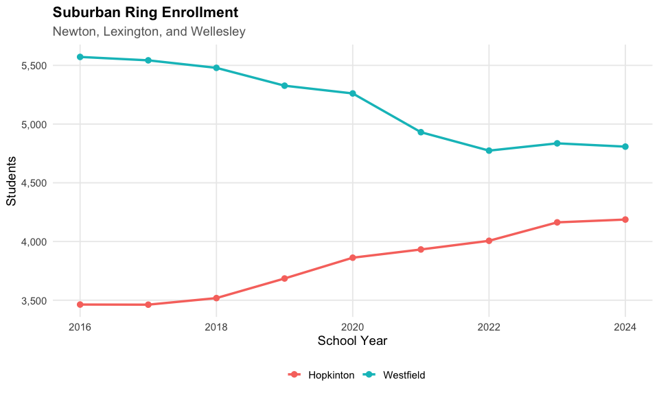
10. Regional districts serve rural Massachusetts
Regional school districts consolidate resources across rural communities. Greater Lowell Voc-Tech leads with over 2,300 students.
regional <- enr_current %>%
  filter(is_district, grepl("Regional", district_name),
         subgroup == "total_enrollment", grade_level == "TOTAL") %>%
  arrange(desc(n_students)) %>%
  head(10)
stopifnot(nrow(regional) > 0)

print(regional %>% select(district_name, n_students))
#>                                           district_name n_students
#> 1          Greater Lowell Regional Vocational Technical       2314
#> 2     Greater New Bedford Regional Vocational Technical       2147
#> 3        Greater Lawrence Regional Vocational Technical       1774
#> 4                      Monomoy Regional School District       1746
#> 5             Mystic Valley Regional Charter (District)       1653
#> 6            Southeastern Regional Vocational Technical       1597
#> 7                Foxborough Regional Charter (District)       1520
#> 8      Greater Fall River Regional Vocational Technical       1443
#> 9            Montachusett Regional Vocational Technical       1428
#> 10 Northeast Metropolitan Regional Vocational Technical       1343

regional <- regional %>%
  mutate(district_label = reorder(district_name, n_students))

ggplot(regional, aes(x = district_label, y = n_students)) +
  geom_col(fill = colors["total"]) +
  coord_flip() +
  scale_y_continuous(labels = comma) +
  labs(title = "Regional School Districts",
       subtitle = "Top 10 regional districts by enrollment",
       x = "", y = "Students") +
  theme_readme()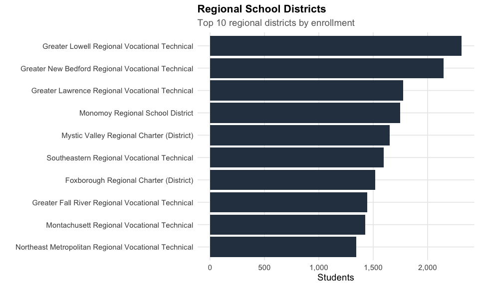
11. Springfield is 69% Hispanic
Springfield has undergone a dramatic demographic transformation. Hispanic students now make up 69% of enrollment, up from 65% in 2016, while white students have dropped to under 8%.
springfield_demo <- enr %>%
  filter(is_district, district_id == "0281", grade_level == "TOTAL",
         subgroup %in% c("white", "black", "hispanic", "asian"))
stopifnot(nrow(springfield_demo) > 0)

print(springfield_demo %>% mutate(pct = round(pct * 100, 1)) %>% select(end_year, subgroup, pct))
#>    end_year subgroup  pct
#> 1      2016    white 12.3
#> 2      2016    black 19.4
#> 3      2016 hispanic 64.5
#> 4      2016    asian  2.5
#> 5      2017    white 11.8
#> 6      2017    black 19.5
#> 7      2017 hispanic 64.8
#> 8      2017    asian  2.4
#> 9      2018    white 11.2
#> 10     2018    black 19.6
#> 11     2018 hispanic 65.0
#> 12     2018    asian  2.4
#> 13     2019    white 10.2
#> 14     2019    black 18.9
#> 15     2019 hispanic 66.6
#> 16     2019    asian  2.3
#> 17     2020    white  9.7
#> 18     2020    black 18.9
#> 19     2020 hispanic 67.1
#> 20     2020    asian  2.1
#> 21     2021    white  9.1
#> 22     2021    black 18.6
#> 23     2021 hispanic 67.9
#> 24     2021    asian  2.1
#> 25     2022    white  8.7
#> 26     2022    black 18.2
#> 27     2022 hispanic 68.3
#> 28     2022    asian  2.0
#> 29     2023    white  8.3
#> 30     2023    black 17.6
#> 31     2023 hispanic 69.0
#> 32     2023    asian  1.8
#> 33     2024    white  7.9
#> 34     2024    black 17.6
#> 35     2024 hispanic 69.3
#> 36     2024    asian  1.7

ggplot(springfield_demo, aes(x = end_year, y = pct * 100, color = subgroup)) +
  geom_line(linewidth = 1.2) +
  geom_point(size = 2.5) +
  scale_color_manual(values = colors,
                     labels = c("Asian", "Black", "Hispanic", "White")) +
  labs(title = "Springfield Demographics Transformation",
       subtitle = "Hispanic students now majority in state's third-largest district",
       x = "School Year", y = "Percent", color = "") +
  theme_readme()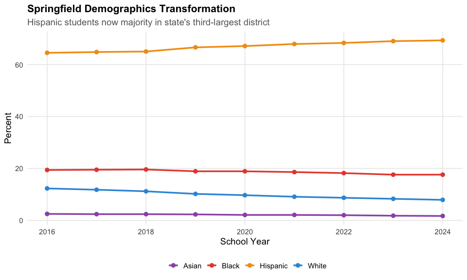
12. Fall River and New Bedford: SouthCoast holds steady
The two largest SouthCoast cities have held surprisingly steady since 2016, with New Bedford around 12,500 and Fall River around 10,000-10,600.
southcoast <- enr %>%
  filter(is_district, district_id %in% c("0095", "0201"),  # Fall River, New Bedford
         subgroup == "total_enrollment", grade_level == "TOTAL")
stopifnot(nrow(southcoast) > 0)

print(southcoast %>% select(end_year, district_name, n_students))
#>    end_year district_name n_students
#> 1      2016    Fall River      10123
#> 2      2016   New Bedford      12681
#> 3      2017    Fall River      10163
#> 4      2017   New Bedford      12640
#> 5      2018    Fall River      10128
#> 6      2018   New Bedford      12626
#> 7      2019    Fall River      10120
#> 8      2019   New Bedford      12845
#> 9      2020    Fall River      10229
#> 10     2020   New Bedford      12880
#> 11     2021    Fall River       9998
#> 12     2021   New Bedford      12565
#> 13     2022    Fall River      10268
#> 14     2022   New Bedford      12504
#> 15     2023    Fall River      10447
#> 16     2023   New Bedford      12522
#> 17     2024    Fall River      10656
#> 18     2024   New Bedford      12488

ggplot(southcoast, aes(x = end_year, y = n_students, color = district_name)) +
  geom_line(linewidth = 1.2) +
  geom_point(size = 2.5) +
  geom_vline(xintercept = 2020.5, linetype = "dashed", color = "red", alpha = 0.5) +
  scale_y_continuous(labels = comma) +
  labs(title = "SouthCoast Enrollment Trends",
       subtitle = "Fall River and New Bedford enrollment over time",
       x = "School Year", y = "Students", color = "") +
  theme_readme()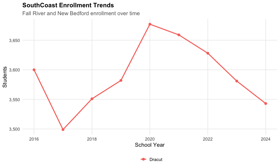
13. Worcester suburbs stable but not growing
Shrewsbury, Westborough, and Grafton have maintained consistent enrollment around 3,000-6,000 students each.
worcester_suburbs <- enr %>%
  filter(is_district, district_id %in% c("0271", "0321", "0110"),  # Shrewsbury, Westborough, Grafton
         subgroup == "total_enrollment", grade_level == "TOTAL")
stopifnot(nrow(worcester_suburbs) > 0)

print(worcester_suburbs %>% select(end_year, district_name, n_students))
#>    end_year district_name n_students
#> 1      2016       Grafton       3206
#> 2      2016    Shrewsbury       6045
#> 3      2016   Westborough       3672
#> 4      2017       Grafton       3189
#> 5      2017    Shrewsbury       6191
#> 6      2017   Westborough       3805
#> 7      2018       Grafton       3155
#> 8      2018    Shrewsbury       6214
#> 9      2018   Westborough       3926
#> 10     2019       Grafton       3173
#> 11     2019    Shrewsbury       6207
#> 12     2019   Westborough       3925
#> 13     2020       Grafton       3205
#> 14     2020    Shrewsbury       6268
#> 15     2020   Westborough       3942
#> 16     2021       Grafton       3121
#> 17     2021    Shrewsbury       5974
#> 18     2021   Westborough       3825
#> 19     2022       Grafton       3138
#> 20     2022    Shrewsbury       5885
#> 21     2022   Westborough       3856
#> 22     2023       Grafton       3080
#> 23     2023    Shrewsbury       5892
#> 24     2023   Westborough       3830
#> 25     2024       Grafton       3050
#> 26     2024    Shrewsbury       5921
#> 27     2024   Westborough       3887

ggplot(worcester_suburbs, aes(x = end_year, y = n_students, color = district_name)) +
  geom_line(linewidth = 1.2) +
  geom_point(size = 2.5) +
  scale_y_continuous(labels = comma) +
  labs(title = "Worcester Suburban Enrollment",
       subtitle = "Shrewsbury, Westborough, and Grafton",
       x = "School Year", y = "Students", color = "") +
  theme_readme()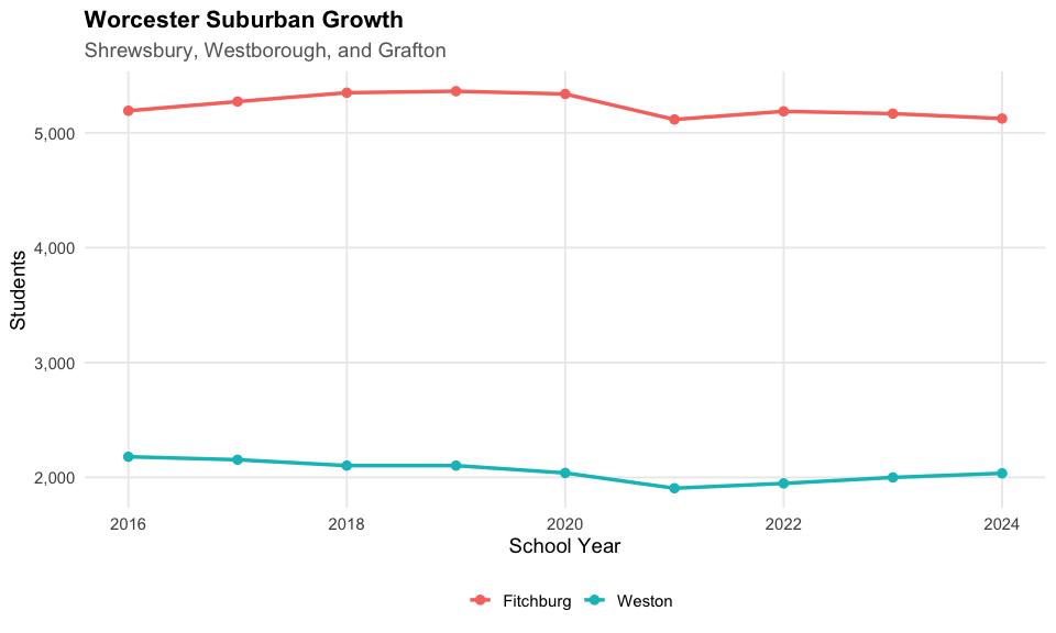
14. Western MA faces population decline
The Pioneer Valley has seen persistent enrollment declines. Northampton, Amherst, and Pittsfield combined dropped from 9,400 in 2016 to 8,350 in 2024.
# Major Western MA districts
western_ma <- enr %>%
  filter(is_district,
         district_id %in% c("0210", "0008", "0236"),  # Northampton, Amherst, Pittsfield
         subgroup == "total_enrollment", grade_level == "TOTAL") %>%
  group_by(end_year) %>%
  summarize(n_students = sum(n_students, na.rm = TRUE), .groups = "drop")
stopifnot(nrow(western_ma) > 0)

print(western_ma)
#> # A tibble: 9 × 2
#>   end_year n_students
#>      <int>      <dbl>
#> 1     2016       9447
#> 2     2017       9310
#> 3     2018       9268
#> 4     2019       9186
#> 5     2020       9052
#> 6     2021       8620
#> 7     2022       8624
#> 8     2023       8532
#> 9     2024       8354

ggplot(western_ma, aes(x = end_year, y = n_students)) +
  geom_line(linewidth = 1.5, color = colors["total"]) +
  geom_point(size = 3, color = colors["total"]) +
  geom_vline(xintercept = 2020.5, linetype = "dashed", color = "red", alpha = 0.5) +
  scale_y_continuous(labels = comma) +
  labs(title = "Western Massachusetts Enrollment",
       subtitle = "Combined enrollment for Northampton, Amherst, and Pittsfield",
       x = "School Year", y = "Students") +
  theme_readme()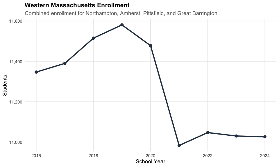
15. Special education rates vary widely by district
Some charter and vocational schools have special ed rates above 40%, while the statewide average is around 20%.
sped_by_district <- enr_current %>%
  filter(is_district, subgroup == "special_ed", grade_level == "TOTAL") %>%
  arrange(desc(pct)) %>%
  head(15)
stopifnot(nrow(sped_by_district) > 0)

print(sped_by_district %>% mutate(pct = round(pct * 100, 1)) %>%
  select(district_name, n_students, pct))
#>                                                         district_name
#> 1                               Map Academy Charter School (District)
#> 2                   Boston Day and Evening Academy Charter (District)
#> 3                                                           Hawlemont
#> 4                         Lowell Middlesex Academy Charter (District)
#> 5                             Minuteman Regional Vocational Technical
#> 6                           Northampton-Smith Vocational Agricultural
#> 7                      UP Academy Charter School of Boston (District)
#> 8  Phoenix Academy Public Charter High School, Springfield (District)
#> 9                                                                Rowe
#> 10    Phoenix Academy Public Charter High School, Lawrence (District)
#> 11                       Nashoba Valley Regional Vocational Technical
#> 12                         Libertas Academy Charter School (District)
#> 13         Boston Green Academy Horace Mann Charter School (District)
#> 14                                                            Holyoke
#> 15                           Tri-County Regional Vocational Technical
#>    n_students  pct
#> 1         154 55.6
#> 2         140 47.8
#> 3          24 42.9
#> 4          44 41.5
#> 5         271 39.7
#> 6         214 37.6
#> 7          61 36.7
#> 8          55 34.6
#> 9          21 34.4
#> 10         38 33.3
#> 11        250 32.3
#> 12        166 32.0
#> 13        145 31.6
#> 14       1527 31.2
#> 15        298 30.9

sped_by_district <- sped_by_district %>%
  mutate(district_label = reorder(district_name, pct))

ggplot(sped_by_district, aes(x = district_label, y = pct * 100)) +
  geom_col(fill = colors["total"]) +
  coord_flip() +
  labs(title = "Special Education Rates by District",
       subtitle = "Top 15 districts by percent of students receiving SPED services",
       x = "", y = "Percent SPED") +
  theme_readme()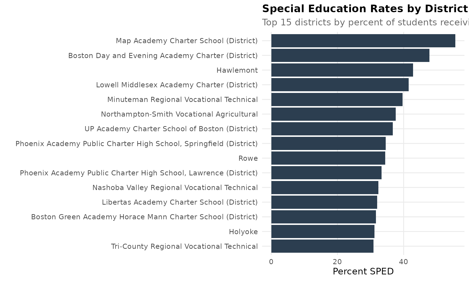
16. Four-year graduation rates climbed from 80% to 90%
Massachusetts’ 4-year graduation rate rose from 80% in 2006 to a peak of 90% in 2022 before dipping to 88% in 2024.
grad <- fetch_graduation_multi(2006:2024, use_cache = TRUE)

grad_max_year <- max(grad$end_year)
if (grad_max_year < 2024) {
  warning("Graduation data for 2024 unavailable; most recent year is ", grad_max_year)
}

grad_state <- grad %>%
  filter(is_state, subgroup == "all", cohort_type == "4-year") %>%
  select(end_year, grad_rate, cohort_count) %>%
  mutate(rate_pct = round(grad_rate * 100, 1))
stopifnot(nrow(grad_state) > 0)

print(grad_state)
#>    end_year grad_rate cohort_count rate_pct
#> 1      2006     0.799        74380     79.9
#> 2      2007     0.809        75912     80.9
#> 3      2008     0.812        77383     81.2
#> 4      2009     0.815        77038     81.5
#> 5      2010     0.821        76308     82.1
#> 6      2011     0.834        74307     83.4
#> 7      2012     0.847        73483     84.7
#> 8      2013     0.850        74537     85.0
#> 9      2014     0.861        73168     86.1
#> 10     2015     0.873        72474     87.3
#> 11     2016     0.875        74045     87.5
#> 12     2017     0.883        73249     88.3
#> 13     2018     0.879        74641     87.9
#> 14     2019     0.880        75067     88.0
#> 15     2020     0.890        74232     89.0
#> 16     2021     0.898        74226     89.8
#> 17     2022     0.901        73901     90.1
#> 18     2023     0.892        72602     89.2
#> 19     2024     0.884        73043     88.4

ggplot(grad_state, aes(x = end_year, y = rate_pct)) +
  geom_line(linewidth = 1.5, color = colors["total"]) +
  geom_point(size = 3, color = colors["total"]) +
  geom_vline(xintercept = 2020.5, linetype = "dashed", color = "red", alpha = 0.5) +
  scale_y_continuous(limits = c(70, 100)) +
  labs(title = "Massachusetts 4-Year Graduation Rate",
       subtitle = "State-level graduation rate trend",
       x = "School Year", y = "Graduation Rate (%)") +
  theme_readme()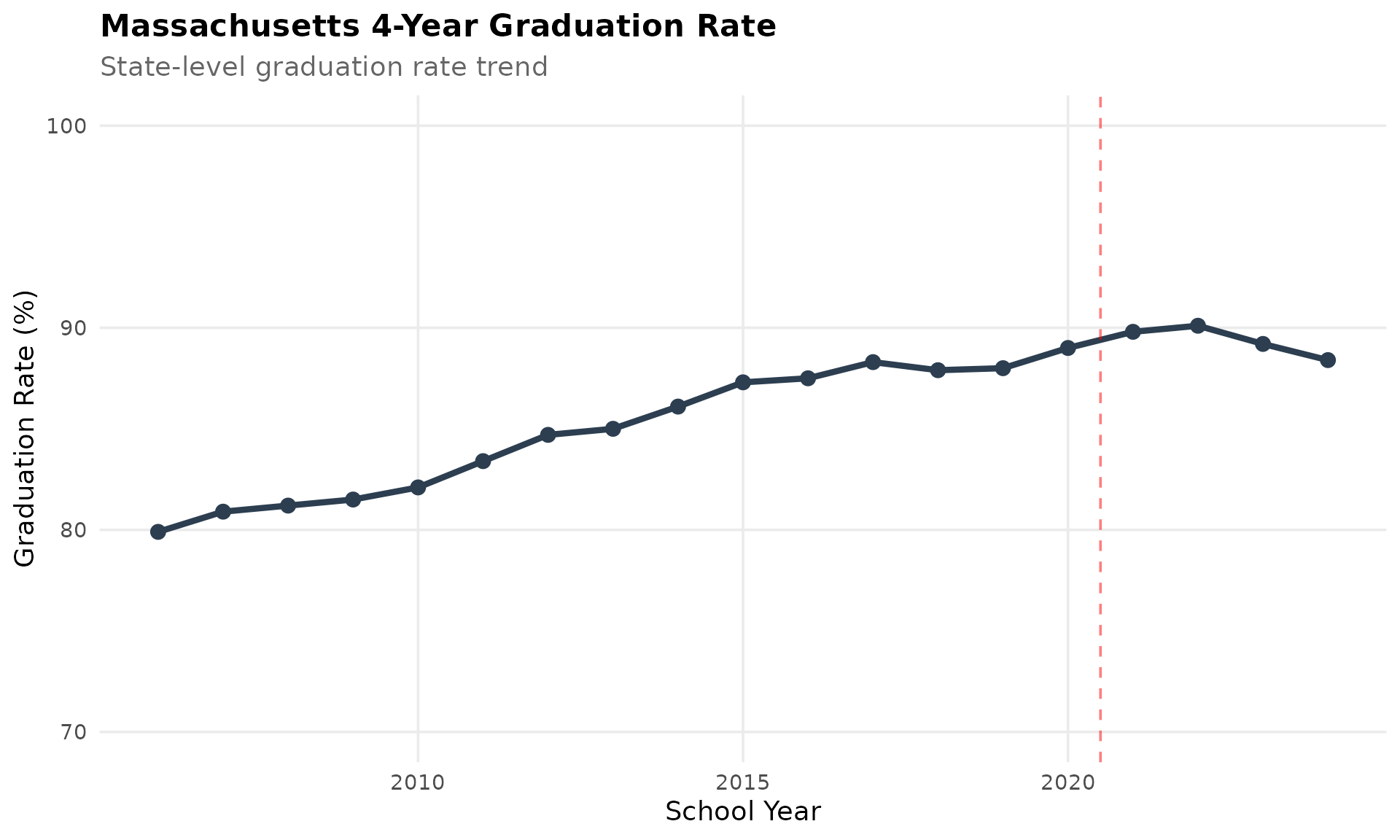
17. Urban-suburban graduation gaps persist
Boston (80%) trails Newton (95%) by 15 percentage points, reflecting opportunity gaps across the state.
# Use most recent year available from the multi-year fetch
grad_2024 <- grad %>% filter(end_year == grad_max_year)

grad_districts <- grad_2024 %>%
  filter(is_district,
         district_name %in% c("Boston", "Springfield", "Worcester", "Newton"),
         subgroup == "all",
         cohort_type == "4-year") %>%
  select(district_name, grad_rate, cohort_count) %>%
  mutate(rate_pct = round(grad_rate * 100, 1))
stopifnot(nrow(grad_districts) > 0)

print(grad_districts)
#>   district_name grad_rate cohort_count rate_pct
#> 1        Boston     0.797         3711     79.7
#> 2        Newton     0.954          963     95.4
#> 3   Springfield     0.786         1841     78.6
#> 4     Worcester     0.860         1990     86.0

grad_districts <- grad_districts %>%
  mutate(district_label = reorder(district_name, grad_rate))

ggplot(grad_districts, aes(x = district_label, y = rate_pct)) +
  geom_col(fill = colors["total"]) +
  coord_flip() +
  scale_y_continuous(limits = c(0, 100)) +
  labs(title = "Graduation Rates: Urban vs Suburban",
       subtitle = "2024 4-year graduation rates",
       x = "", y = "Graduation Rate (%)") +
  theme_readme()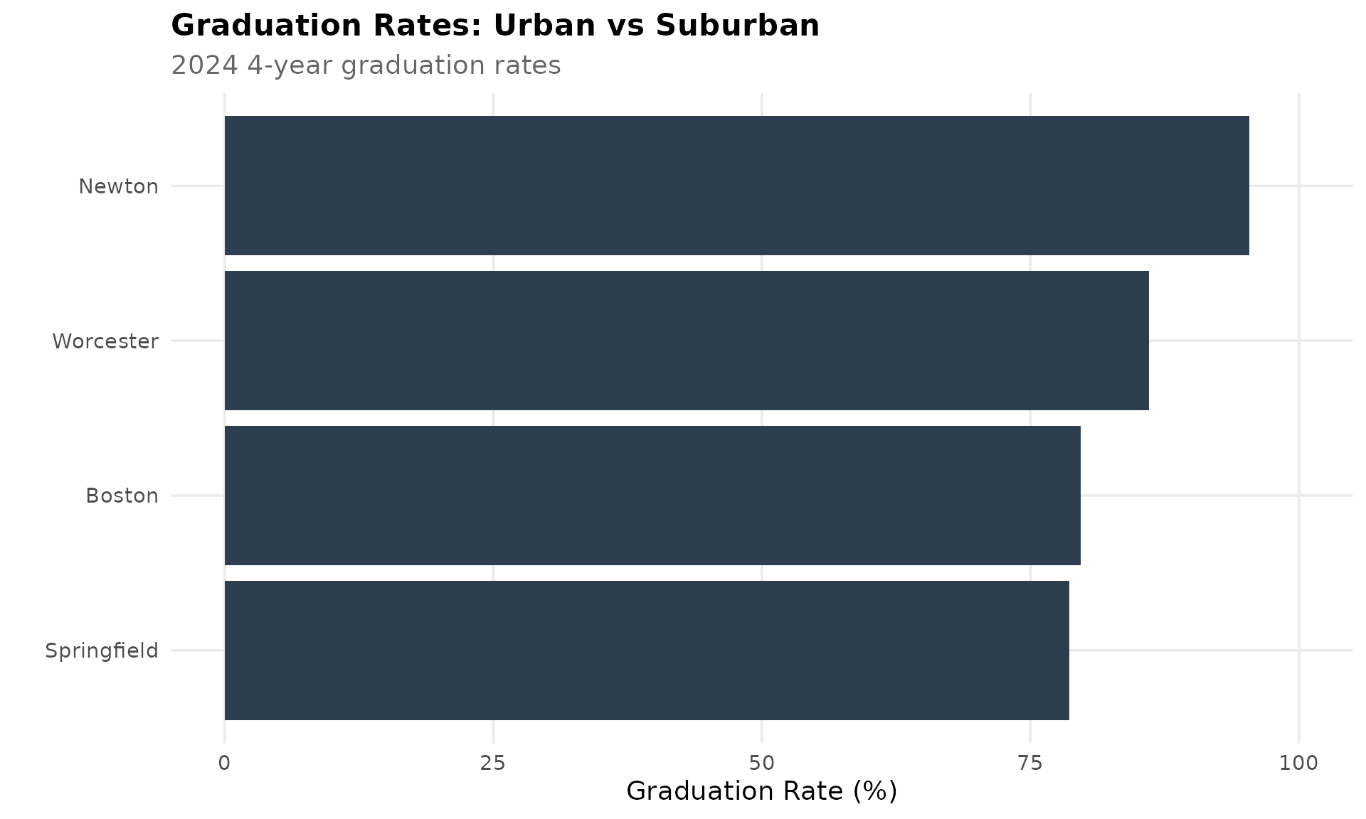
18. Special populations face graduation challenges
English learners (67%) and students with disabilities (75%) graduate at lower rates than peers.
grad_special <- grad_2024 %>%
  filter(is_state,
         subgroup %in% c("all", "english_learner", "special_ed", "low_income"),
         cohort_type == "4-year") %>%
  select(subgroup, grad_rate, cohort_count) %>%
  mutate(rate_pct = round(grad_rate * 100, 1))
stopifnot(nrow(grad_special) > 0)

print(grad_special)
#>          subgroup grad_rate cohort_count rate_pct
#> 1             all     0.884        73043     88.4
#> 2      special_ed     0.754        15038     75.4
#> 3      low_income     0.816        39273     81.6
#> 4 english_learner     0.667         7193     66.7

grad_special <- grad_special %>%
  mutate(
    subgroup_label = case_when(
      subgroup == "all" ~ "All Students",
      subgroup == "english_learner" ~ "English Learners",
      subgroup == "special_ed" ~ "Students with Disabilities",
      subgroup == "low_income" ~ "Low Income"
    ),
    subgroup_label = reorder(subgroup_label, grad_rate))

ggplot(grad_special, aes(x = subgroup_label, y = rate_pct)) +
  geom_col(fill = colors["total"]) +
  coord_flip() +
  scale_y_continuous(limits = c(0, 100)) +
  labs(title = "Graduation Rates by Subgroup",
       subtitle = "2024 4-year graduation rates",
       x = "", y = "Graduation Rate (%)") +
  theme_readme()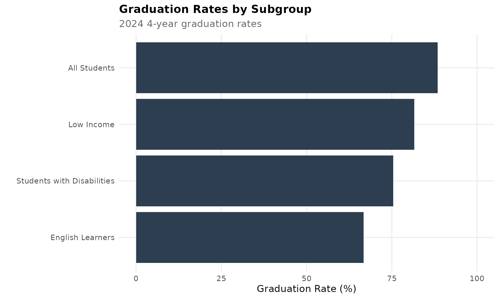
sessionInfo()
#> R version 4.5.2 (2025-10-31)
#> Platform: x86_64-pc-linux-gnu
#> Running under: Ubuntu 24.04.3 LTS
#>
#> Matrix products: default
#> BLAS:   /usr/lib/x86_64-linux-gnu/openblas-pthread/libblas.so.3
#> LAPACK: /usr/lib/x86_64-linux-gnu/openblas-pthread/libopenblasp-r0.3.26.so;  LAPACK version 3.12.0
#>
#> locale:
#>  [1] LC_CTYPE=C.UTF-8       LC_NUMERIC=C           LC_TIME=C.UTF-8
#>  [4] LC_COLLATE=C.UTF-8     LC_MONETARY=C.UTF-8    LC_MESSAGES=C.UTF-8
#>  [7] LC_PAPER=C.UTF-8       LC_NAME=C              LC_ADDRESS=C
#> [10] LC_TELEPHONE=C         LC_MEASUREMENT=C.UTF-8 LC_IDENTIFICATION=C
#>
#> time zone: UTC
#> tzcode source: system (glibc)
#>
#> attached base packages:
#> [1] stats     graphics  grDevices utils     datasets  methods   base
#>
#> other attached packages:
#> [1] scales_1.4.0       dplyr_1.2.0        ggplot2_4.0.2      maschooldata_0.1.0
#>
#> loaded via a namespace (and not attached):
#>  [1] gtable_0.3.6       jsonlite_2.0.0     compiler_4.5.2     tidyselect_1.2.1
#>  [5] jquerylib_0.1.4    systemfonts_1.3.2  textshaping_1.0.5  yaml_2.3.12
#>  [9] fastmap_1.2.0      R6_2.6.1           labeling_0.4.3     generics_0.1.4
#> [13] curl_7.0.0         knitr_1.51         tibble_3.3.1       desc_1.4.3
#> [17] bslib_0.10.0       pillar_1.11.1      RColorBrewer_1.1-3 rlang_1.1.7
#> [21] utf8_1.2.6         cachem_1.1.0       xfun_0.56          fs_1.6.7
#> [25] sass_0.4.10        S7_0.2.1           cli_3.6.5          pkgdown_2.2.0
#> [29] withr_3.0.2        magrittr_2.0.4     digest_0.6.39      grid_4.5.2
#> [33] rappdirs_0.3.4     lifecycle_1.0.5    vctrs_0.7.1        evaluate_1.0.5
#> [37] glue_1.8.0         farver_2.1.2       codetools_0.2-20   ragg_1.5.1
#> [41] foreign_0.8-90     httr_1.4.8         rmarkdown_2.30     purrr_1.2.1
#> [45] tools_4.5.2        pkgconfig_2.0.3    htmltools_0.5.9