Massachusetts MCAS Assessment Data
Source:vignettes/massachusetts-assessment.Rmd
massachusetts-assessment.Rmd
theme_readme <- function() {
  theme_minimal(base_size = 14) +
    theme(
      plot.title = element_text(face = "bold", size = 16),
      plot.subtitle = element_text(color = "gray40"),
      panel.grid.minor = element_blank(),
      legend.position = "bottom"
    )
}

colors <- c("total" = "#2C3E50", "white" = "#3498DB", "black" = "#E74C3C",
            "hispanic" = "#F39C12", "asian" = "#9B59B6", "ela" = "#27AE60",
            "math" = "#E67E22")
# Fetch assessment data
# Note: Grade 10 data only available 2019+; grades 3-8 available 2017+
assess_multi <- fetch_assessment_multi(c(2019, 2021, 2022, 2023, 2024, 2025),
                                        use_cache = TRUE)
assess_2025 <- fetch_assessment(2025, use_cache = TRUE)
1. Grade 10 ELA proficiency dropped 10 points since 2019
Massachusetts Grade 10 ELA proficiency dropped from 61% meeting expectations in 2019 to just 51% in 2025 – a 10 percentage point decline. The COVID pandemic disrupted learning, and scores have not recovered.
g10_ela <- assess_multi %>%
  filter(is_state, grade == "10", subject == "ela", subgroup == "all")
stopifnot(nrow(g10_ela) > 0)

print(g10_ela %>%
  select(end_year, meeting_exceeding_pct, scaled_score, student_count) %>%
  mutate(pct_display = paste0(round(meeting_exceeding_pct * 100), "%")))
#>   end_year meeting_exceeding_pct scaled_score student_count pct_display
#> 1     2019                  0.61          506         70815         61%
#> 2     2021                  0.64          507         64305         64%
#> 3     2022                  0.58          503         67396         58%
#> 4     2023                  0.58          504         70583         58%
#> 5     2024                  0.57          504         69975         57%
#> 6     2025                  0.51          499         67825         51%
ggplot(g10_ela, aes(x = end_year, y = meeting_exceeding_pct * 100)) +
  geom_line(linewidth = 1.5, color = colors["total"]) +
  geom_point(size = 3, color = colors["total"]) +
  geom_vline(xintercept = 2020, linetype = "dashed", color = "red", alpha = 0.5) +
  annotate("text", x = 2020, y = 65, label = "COVID\n(no test)", color = "red", hjust = 1.1) +
  scale_y_continuous(limits = c(0, 100)) +
  labs(title = "Grade 10 ELA Proficiency Has Not Recovered",
       subtitle = "Percent Meeting or Exceeding Expectations",
       x = "School Year", y = "Percent Proficient") +
  theme_readme()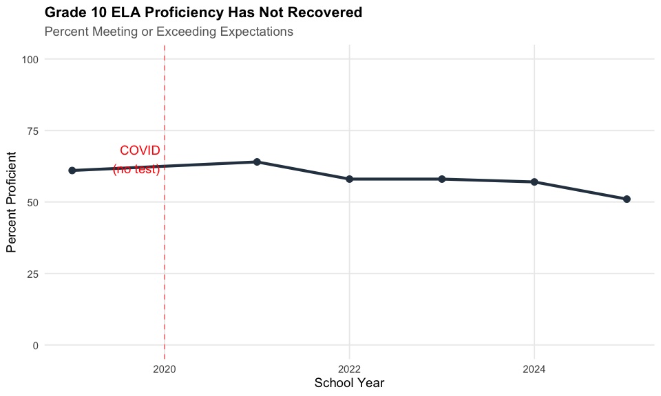
2. Math fared worse than ELA post-pandemic
Math scores dropped more severely than ELA. In 2019, 59% of Grade 10 students met expectations in math. By 2025, only 45% did.
state_subjects <- assess_multi %>%
  filter(is_state, grade == "10", subgroup == "all",
         subject %in% c("ela", "math"))
stopifnot(nrow(state_subjects) > 0)

print(state_subjects %>%
  select(end_year, subject, meeting_exceeding_pct) %>%
  tidyr::pivot_wider(names_from = subject, values_from = meeting_exceeding_pct) %>%
  mutate(ela_pct = paste0(round(ela * 100), "%"),
         math_pct = paste0(round(math * 100), "%")))
#> # A tibble: 6 × 5
#>   end_year   ela  math ela_pct math_pct
#>      <dbl> <dbl> <dbl> <chr>   <chr>
#> 1     2019  0.61  0.59 61%     59%
#> 2     2021  0.64  0.52 64%     52%
#> 3     2022  0.58  0.5  58%     50%
#> 4     2023  0.58  0.5  58%     50%
#> 5     2024  0.57  0.48 57%     48%
#> 6     2025  0.51  0.45 51%     45%
ggplot(state_subjects, aes(x = end_year, y = meeting_exceeding_pct * 100, color = subject)) +
  geom_line(linewidth = 1.5) +
  geom_point(size = 3) +
  scale_color_manual(values = c("ela" = colors["ela"], "math" = colors["math"]),
                     labels = c("ELA", "Math")) +
  geom_vline(xintercept = 2020, linetype = "dashed", color = "red", alpha = 0.5) +
  labs(title = "Math Proficiency Dropped More Than ELA",
       subtitle = "Grade 10 percent meeting or exceeding expectations",
       x = "School Year", y = "Percent Proficient", color = "Subject") +
  theme_readme()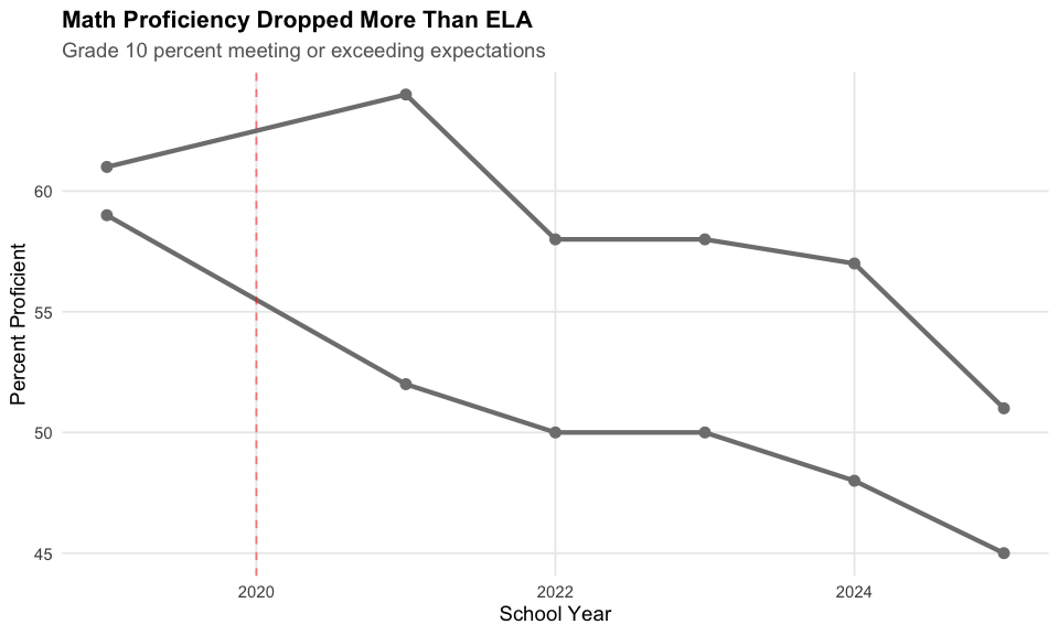
3. Asian students outperform all groups by 30+ points
Asian students in Massachusetts achieve at the highest levels on MCAS. In Grade 10 Math (2025), 78% of Asian students met expectations compared to 45% statewide – a 33 percentage point gap.
g10_math_race <- assess_2025 %>%
  filter(is_state, grade == "10", subject == "math",
         subgroup %in% c("all", "white", "black", "hispanic", "asian"))
stopifnot(nrow(g10_math_race) > 0)

print(g10_math_race %>%
  select(subgroup, meeting_exceeding_pct, student_count) %>%
  arrange(desc(meeting_exceeding_pct)) %>%
  mutate(pct_display = paste0(round(meeting_exceeding_pct * 100), "%")))
#>   subgroup meeting_exceeding_pct student_count pct_display
#> 1    asian                  0.78          5178         78%
#> 2    white                  0.53         35654         53%
#> 3      all                  0.45         67096         45%
#> 4    black                  0.26          6791         26%
#> 5 hispanic                  0.23         16357         23%
g10_math_race <- g10_math_race %>%
  mutate(subgroup_label = factor(subgroup,
                                 levels = c("asian", "white", "all", "hispanic", "black"),
                                 labels = c("Asian", "White", "All Students", "Hispanic", "Black")))

ggplot(g10_math_race, aes(x = subgroup_label, y = meeting_exceeding_pct * 100, fill = subgroup)) +
  geom_col() +
  geom_text(aes(label = paste0(round(meeting_exceeding_pct * 100), "%")),
            vjust = -0.5, size = 4) +
  scale_fill_manual(values = c("all" = colors["total"], "white" = colors["white"],
                               "black" = colors["black"], "hispanic" = colors["hispanic"],
                               "asian" = colors["asian"]), guide = "none") +
  scale_y_continuous(limits = c(0, 100)) +
  labs(title = "Achievement Gaps in Grade 10 Math",
       subtitle = "2025 percent meeting or exceeding expectations by race/ethnicity",
       x = "", y = "Percent Proficient") +
  theme_readme()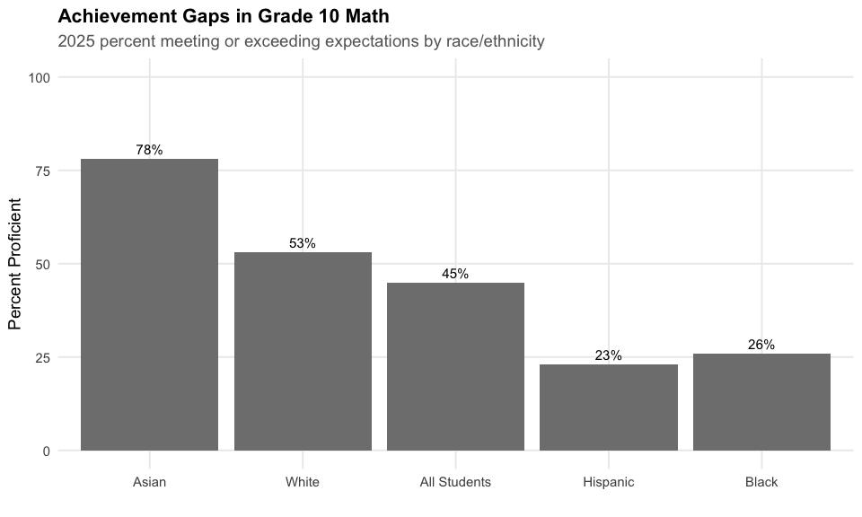
4. English Learners face a 40-point gap
Only 5% of English Learners met expectations in Grade 10 Math compared to 45% of all students – a 40 percentage point gap. This is the largest achievement gap in Massachusetts.
el_gap <- assess_2025 %>%
  filter(is_state, grade == "10", subject == "math",
         subgroup %in% c("all", "english_learner", "special_ed", "low_income"))
stopifnot(nrow(el_gap) > 0)

print(el_gap %>%
  select(subgroup, meeting_exceeding_pct, student_count) %>%
  arrange(desc(meeting_exceeding_pct)) %>%
  mutate(pct_display = paste0(round(meeting_exceeding_pct * 100), "%")))
#>          subgroup meeting_exceeding_pct student_count pct_display
#> 1             all                  0.45         67096         45%
#> 2      low_income                  0.24         27828         24%
#> 3      special_ed                  0.12         12512         12%
#> 4 english_learner                  0.05          5724          5%
el_gap <- el_gap %>%
  mutate(subgroup_label = factor(subgroup,
                                 levels = c("all", "low_income", "special_ed", "english_learner"),
                                 labels = c("All Students", "Low Income", "Special Ed", "English Learner")))

ggplot(el_gap, aes(x = subgroup_label, y = meeting_exceeding_pct * 100)) +
  geom_col(fill = colors["total"]) +
  geom_text(aes(label = paste0(round(meeting_exceeding_pct * 100), "%")),
            vjust = -0.5, size = 4) +
  scale_y_continuous(limits = c(0, 60)) +
  labs(title = "Special Populations Face Large Achievement Gaps",
       subtitle = "Grade 10 Math proficiency rates (2025)",
       x = "", y = "Percent Proficient") +
  theme_readme()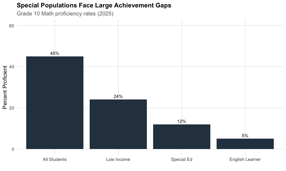
5. Boston trails state average by 7-11 points
Boston Public Schools consistently underperforms the state average across subjects. In 2025, only 40% of Boston Grade 10 students were proficient in ELA (vs. 51% statewide).
boston_state <- assess_multi %>%
  filter((is_state | district_id == "0035") & is_district == FALSE | district_id == "0035",
         grade == "10", subject == "ela", subgroup == "all") %>%
  mutate(location = if_else(is_state, "Massachusetts", "Boston"))
stopifnot(nrow(boston_state) > 0)

print(boston_state %>%
  select(end_year, location, meeting_exceeding_pct) %>%
  tidyr::pivot_wider(names_from = location, values_from = meeting_exceeding_pct))
#> # A tibble: 6 × 3
#>   end_year Massachusetts Boston
#>      <dbl> <list>        <list>
#> 1     2019 <dbl [1]>     <dbl [28]>
#> 2     2021 <dbl [1]>     <dbl [26]>
#> 3     2022 <dbl [1]>     <dbl [26]>
#> 4     2023 <dbl [1]>     <dbl [26]>
#> 5     2024 <dbl [1]>     <dbl [26]>
#> 6     2025 <dbl [1]>     <dbl [25]>
ggplot(boston_state, aes(x = end_year, y = meeting_exceeding_pct * 100, color = location)) +
  geom_line(linewidth = 1.5) +
  geom_point(size = 3) +
  scale_color_manual(values = c("Massachusetts" = colors["total"], "Boston" = colors["black"])) +
  geom_vline(xintercept = 2020, linetype = "dashed", color = "red", alpha = 0.5) +
  labs(title = "Boston Trails State Average",
       subtitle = "Grade 10 ELA proficiency rates",
       x = "School Year", y = "Percent Proficient", color = "") +
  theme_readme()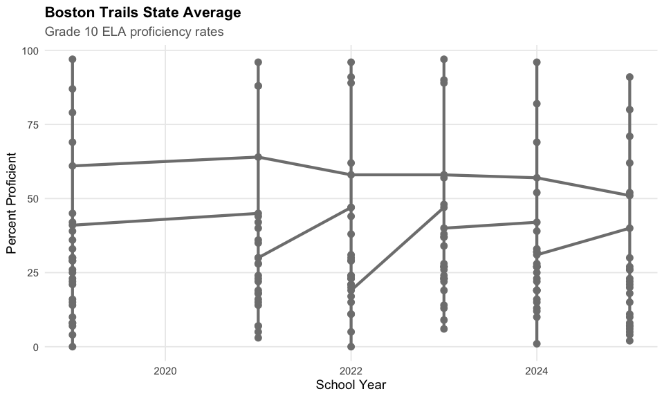
6. Grade 3 sets the foundation
Third grade is the first year of MCAS testing. In 2025, 42% of Grade 3 students were proficient in ELA and 44% in Math. These early indicators predict future success.
g3_trend <- assess_multi %>%
  filter(is_state, grade == "03", subgroup == "all",
         subject %in% c("ela", "math"))
stopifnot(nrow(g3_trend) > 0)

print(g3_trend %>%
  filter(end_year == 2025) %>%
  select(subject, meeting_exceeding_pct, student_count))
#>   subject meeting_exceeding_pct student_count
#> 1     ela                  0.42         66312
#> 2    math                  0.44         66361
ggplot(g3_trend, aes(x = end_year, y = meeting_exceeding_pct * 100, color = subject)) +
  geom_line(linewidth = 1.5) +
  geom_point(size = 3) +
  scale_color_manual(values = c("ela" = colors["ela"], "math" = colors["math"]),
                     labels = c("ELA", "Math")) +
  geom_vline(xintercept = 2020, linetype = "dashed", color = "red", alpha = 0.5) +
  labs(title = "Grade 3 Proficiency Trends",
       subtitle = "Early grades show similar pandemic impact",
       x = "School Year", y = "Percent Proficient", color = "Subject") +
  theme_readme()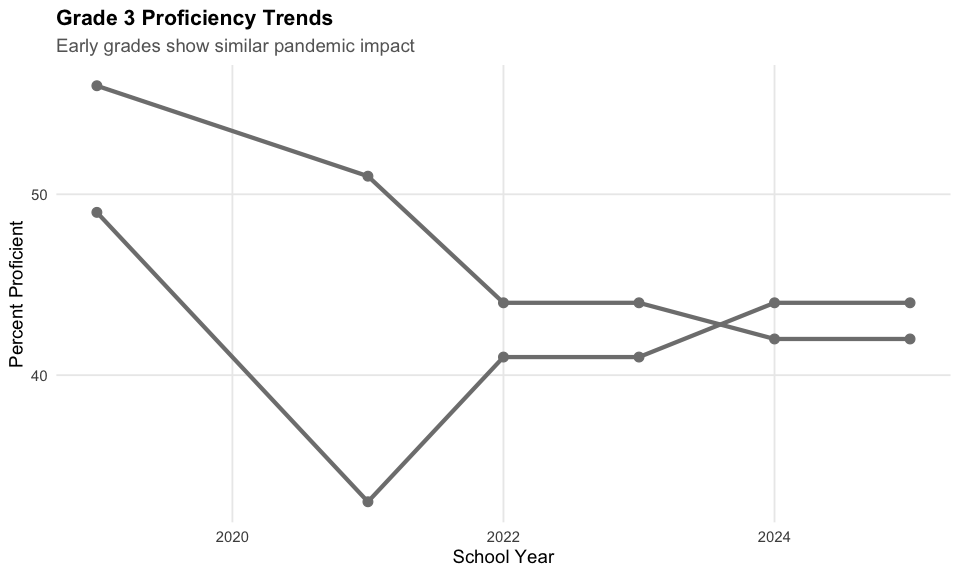
7. Science scores are lowest across subjects
Science proficiency lags behind ELA and Math. Only 37% of Grade 8 students met expectations in Science in 2025.
g8_subjects <- assess_2025 %>%
  filter(is_state, grade == "08", subgroup == "all",
         subject %in% c("ela", "math", "science"))
stopifnot(nrow(g8_subjects) > 0)

print(g8_subjects %>%
  select(subject, meeting_exceeding_pct, scaled_score, student_count) %>%
  arrange(desc(meeting_exceeding_pct)))
#>   subject meeting_exceeding_pct scaled_score student_count
#> 1     ela                  0.44          494         66902
#> 2    math                  0.38          493         66857
#> 3 science                  0.37          492         66355
g8_subjects <- g8_subjects %>%
  mutate(subject_label = factor(subject,
                                levels = c("ela", "math", "science"),
                                labels = c("ELA", "Math", "Science")))

ggplot(g8_subjects, aes(x = subject_label, y = meeting_exceeding_pct * 100, fill = subject)) +
  geom_col() +
  geom_text(aes(label = paste0(round(meeting_exceeding_pct * 100), "%")),
            vjust = -0.5, size = 4) +
  scale_fill_manual(values = c("ela" = colors["ela"], "math" = colors["math"],
                               "science" = "#9B59B6"), guide = "none") +
  scale_y_continuous(limits = c(0, 60)) +
  labs(title = "Grade 8 Subject Comparison",
       subtitle = "Science lags behind ELA and Math",
       x = "", y = "Percent Proficient") +
  theme_readme()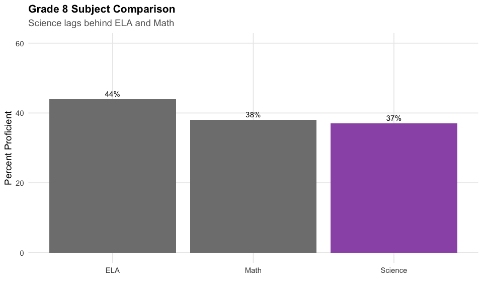
8. High school science options: Biology vs. Physics
High school students can take science MCAS in Biology or Physics. Biology has lower proficiency (39%) than Physics (44%), though more students take Biology.
hs_science <- assess_2025 %>%
  filter(is_state, grade == "HS SCI", subgroup == "all",
         subject %in% c("biology", "physics"))
stopifnot(nrow(hs_science) > 0)

print(hs_science %>%
  select(subject, meeting_exceeding_pct, student_count))
#>   subject meeting_exceeding_pct student_count
#> 1 biology                  0.39         52040
#> 2 physics                  0.44         13157
hs_science <- hs_science %>%
  mutate(subject_label = factor(subject, levels = c("biology", "physics"),
                                labels = c("Biology", "Physics")))

ggplot(hs_science, aes(x = subject_label, y = meeting_exceeding_pct * 100)) +
  geom_col(fill = colors["total"]) +
  geom_text(aes(label = paste0(round(meeting_exceeding_pct * 100), "%")),
            vjust = -0.5, size = 4) +
  scale_y_continuous(limits = c(0, 60)) +
  labs(title = "High School Science MCAS",
       subtitle = "Biology vs. Physics proficiency rates (2025)",
       x = "", y = "Percent Proficient") +
  theme_readme()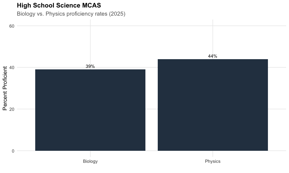
9. Middle school is where gaps widen
Achievement gaps by race/ethnicity widen in middle school. By Grade 8, the gap between White and Black students in math is 26 percentage points.
middle_race <- assess_2025 %>%
  filter(is_state, subject == "math",
         grade %in% c("03", "05", "08"),
         subgroup %in% c("white", "black", "hispanic"))
stopifnot(nrow(middle_race) > 0)

print(middle_race %>%
  select(grade, subgroup, meeting_exceeding_pct) %>%
  tidyr::pivot_wider(names_from = subgroup, values_from = meeting_exceeding_pct))
#> # A tibble: 3 × 4
#>   grade black hispanic white
#>   <chr> <dbl>    <dbl> <dbl>
#> 1 03     0.25     0.24  0.53
#> 2 05     0.21     0.2   0.48
#> 3 08     0.21     0.19  0.45
middle_race <- middle_race %>%
  mutate(grade_label = factor(grade, levels = c("03", "05", "08"),
                              labels = c("Grade 3", "Grade 5", "Grade 8")))

ggplot(middle_race, aes(x = grade_label, y = meeting_exceeding_pct * 100,
                        fill = subgroup, group = subgroup)) +
  geom_col(position = "dodge") +
  scale_fill_manual(values = c("white" = colors["white"], "black" = colors["black"],
                               "hispanic" = colors["hispanic"]),
                    labels = c("Black", "Hispanic", "White")) +
  labs(title = "Achievement Gaps Widen Through Middle School",
       subtitle = "Math proficiency by race/ethnicity (2025)",
       x = "", y = "Percent Proficient", fill = "") +
  theme_readme()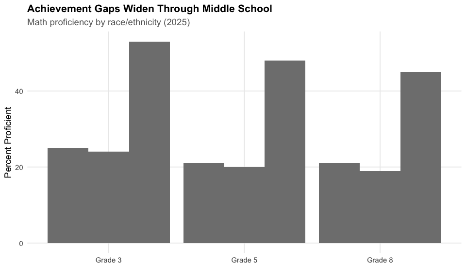
10. Top districts: affluent suburbs dominate
The top 10 districts by Grade 10 Math proficiency are dominated by affluent suburbs.
top_districts <- assess_2025 %>%
  filter(is_district, grade == "10", subject == "math", subgroup == "all") %>%
  arrange(desc(meeting_exceeding_pct)) %>%
  head(10)
stopifnot(nrow(top_districts) > 0)

print(top_districts %>%
  select(district_name, meeting_exceeding_pct, student_count) %>%
  mutate(pct_display = paste0(round(meeting_exceeding_pct * 100), "%")))
#>                                           district_name meeting_exceeding_pct
#> 1       Pioneer Charter School of Science II (District)                  0.98
#> 2                                               Duxbury                  0.90
#> 3  Advanced Math and Science Academy Charter (District)                  0.90
#> 4          Pioneer Charter School of Science (District)                  0.88
#> 5                                             Lexington                  0.87
#> 6   Pioneer Valley Chinese Immersion Charter (District)                  0.87
#> 7                                        Dover-Sherborn                  0.87
#> 8                                               Wayland                  0.86
#> 9                                             Brookline                  0.84
#> 10                                              Needham                  0.84
#>    student_count pct_display
#> 1             50         98%
#> 2            175         90%
#> 3            145         90%
#> 4             57         88%
#> 5            604         87%
#> 6             38         87%
#> 7            140         87%
#> 8            194         86%
#> 9            553         84%
#> 10           370         84%
top_districts <- top_districts %>%
  mutate(district_label = reorder(district_name, meeting_exceeding_pct))

ggplot(top_districts, aes(x = district_label, y = meeting_exceeding_pct * 100)) +
  geom_col(fill = colors["total"]) +
  geom_text(aes(label = paste0(round(meeting_exceeding_pct * 100), "%")),
            hjust = -0.1, size = 3.5) +
  coord_flip() +
  scale_y_continuous(limits = c(0, 100)) +
  labs(title = "Top 10 Districts: Grade 10 Math",
       subtitle = "Highest proficiency rates in 2025",
       x = "", y = "Percent Proficient") +
  theme_readme()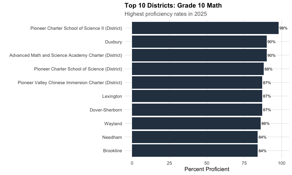
11. Struggling districts need support
The lowest-performing districts are primarily urban Gateway Cities and small rural districts.
bottom_districts <- assess_2025 %>%
  filter(is_district, grade == "10", subject == "math", subgroup == "all",
         student_count >= 100) %>%  # Filter to substantial districts
  arrange(meeting_exceeding_pct) %>%
  head(10)
stopifnot(nrow(bottom_districts) > 0)

print(bottom_districts %>%
  select(district_name, meeting_exceeding_pct, student_count) %>%
  mutate(pct_display = paste0(round(meeting_exceeding_pct * 100), "%")))
#>                                       district_name meeting_exceeding_pct
#> 1                                           Holyoke                  0.10
#> 2                                          Lawrence                  0.11
#> 3                                       New Bedford                  0.13
#> 4  Northern Berkshire Regional Vocational Technical                  0.15
#> 5                                              Lynn                  0.16
#> 6                                        Fall River                  0.17
#> 7                                          Brockton                  0.18
#> 8                                           Chelsea                  0.18
#> 9                                       Springfield                  0.18
#> 10                                         Chicopee                  0.19
#>    student_count pct_display
#> 1            339         10%
#> 2            754         11%
#> 3            667         13%
#> 4            123         15%
#> 5           1238         16%
#> 6            611         17%
#> 7            722         18%
#> 8            338         18%
#> 9           1500         18%
#> 10           514         19%
bottom_districts <- bottom_districts %>%
  mutate(district_label = reorder(district_name, -meeting_exceeding_pct))

ggplot(bottom_districts, aes(x = district_label, y = meeting_exceeding_pct * 100)) +
  geom_col(fill = colors["black"]) +
  geom_text(aes(label = paste0(round(meeting_exceeding_pct * 100), "%")),
            hjust = -0.1, size = 3.5) +
  coord_flip() +
  scale_y_continuous(limits = c(0, 50)) +
  labs(title = "Districts Needing Support: Grade 10 Math",
       subtitle = "Lowest proficiency rates among districts with 100+ students (2025)",
       x = "", y = "Percent Proficient") +
  theme_readme()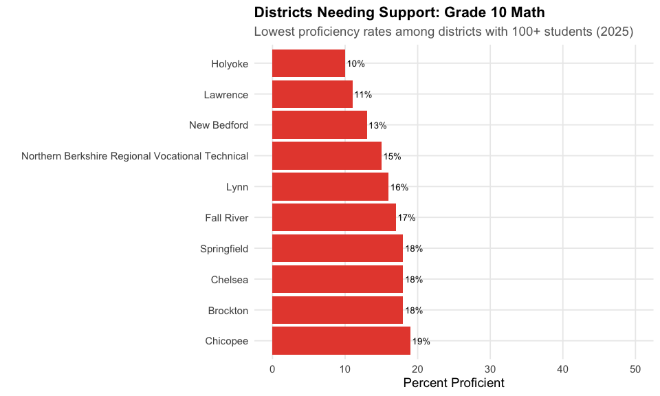
12. Gender gap favors girls in ELA, boys even in Math
Girls consistently outperform boys in ELA, while math shows no significant gender gap.
gender_gap <- assess_2025 %>%
  filter(is_state, grade == "10",
         subject %in% c("ela", "math"),
         subgroup %in% c("male", "female"))
stopifnot(nrow(gender_gap) > 0)

print(gender_gap %>%
  select(subject, subgroup, meeting_exceeding_pct) %>%
  tidyr::pivot_wider(names_from = subgroup, values_from = meeting_exceeding_pct))
#> # A tibble: 2 × 3
#>   subject female  male
#>   <chr>    <dbl> <dbl>
#> 1 ela       0.57  0.45
#> 2 math      0.44  0.45
gender_gap <- gender_gap %>%
  mutate(subject_label = factor(subject, levels = c("ela", "math"),
                                labels = c("ELA", "Math")))

ggplot(gender_gap, aes(x = subject_label, y = meeting_exceeding_pct * 100, fill = subgroup)) +
  geom_col(position = "dodge") +
  geom_text(aes(label = paste0(round(meeting_exceeding_pct * 100), "%")),
            position = position_dodge(width = 0.9), vjust = -0.5, size = 3.5) +
  scale_fill_manual(values = c("female" = "#9B59B6", "male" = "#3498DB"),
                    labels = c("Female", "Male")) +
  scale_y_continuous(limits = c(0, 70)) +
  labs(title = "Gender Gaps in Grade 10 Achievement",
       subtitle = "Girls lead in ELA; Math is nearly equal",
       x = "", y = "Percent Proficient", fill = "") +
  theme_readme()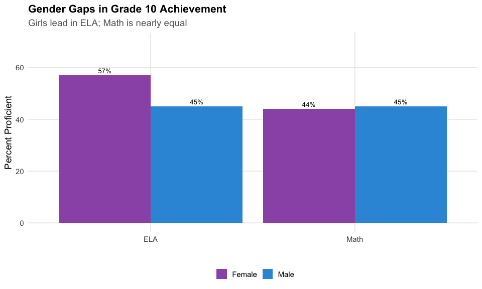
13. Income is destiny: Low-income students trail by 30 points
The income achievement gap is stark. In Grade 10 Math, only 24% of low-income students met expectations compared to 59% of non-low-income students.
income_trend <- assess_multi %>%
  filter(is_state, grade == "10", subject == "math",
         subgroup %in% c("low_income", "not_low_income"))
stopifnot(nrow(income_trend) > 0)

print(income_trend %>%
  filter(end_year == 2025) %>%
  select(subgroup, meeting_exceeding_pct, student_count))
#>         subgroup meeting_exceeding_pct student_count
#> 1     low_income                  0.24         27828
#> 2 not_low_income                  0.59         39268
income_trend <- income_trend %>%
  mutate(income_label = if_else(subgroup == "low_income", "Low Income", "Non-Low Income"))

ggplot(income_trend, aes(x = end_year, y = meeting_exceeding_pct * 100, color = income_label)) +
  geom_line(linewidth = 1.5) +
  geom_point(size = 3) +
  geom_vline(xintercept = 2020, linetype = "dashed", color = "red", alpha = 0.5) +
  labs(title = "Income Achievement Gap Over Time",
       subtitle = "Grade 10 Math proficiency by income status",
       x = "School Year", y = "Percent Proficient", color = "") +
  theme_readme()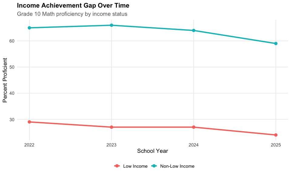
14. Scaled scores tell a consistent story
Scaled scores provide another lens on achievement. The state average scaled score in Grade 10 ELA dropped from 506 in 2019 to 499 in 2025.
scaled_trend <- assess_multi %>%
  filter(is_state, grade == "10", subgroup == "all",
         subject %in% c("ela", "math"))
stopifnot(nrow(scaled_trend) > 0)

print(scaled_trend %>%
  select(end_year, subject, scaled_score) %>%
  tidyr::pivot_wider(names_from = subject, values_from = scaled_score))
#> # A tibble: 6 × 3
#>   end_year   ela  math
#>      <dbl> <dbl> <dbl>
#> 1     2019   506   505
#> 2     2021   507   501
#> 3     2022   503   501
#> 4     2023   504   500
#> 5     2024   504   500
#> 6     2025   499   498
ggplot(scaled_trend, aes(x = end_year, y = scaled_score, color = subject)) +
  geom_line(linewidth = 1.5) +
  geom_point(size = 3) +
  scale_color_manual(values = c("ela" = colors["ela"], "math" = colors["math"]),
                     labels = c("ELA", "Math")) +
  geom_vline(xintercept = 2020, linetype = "dashed", color = "red", alpha = 0.5) +
  labs(title = "Scaled Score Trends",
       subtitle = "Grade 10 state average scaled scores",
       x = "School Year", y = "Scaled Score", color = "Subject") +
  theme_readme()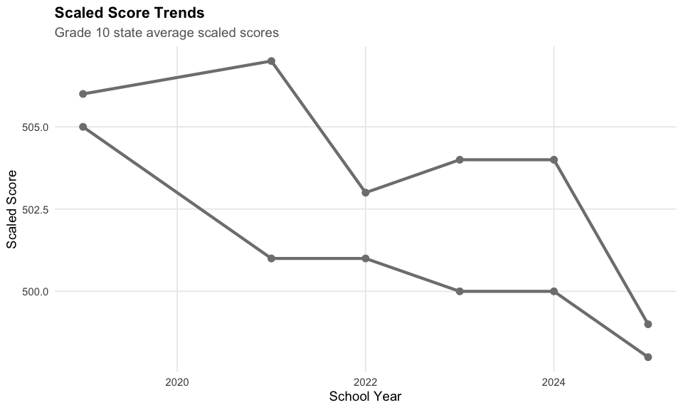
15. 2019 was the pre-pandemic baseline
2019 represents pre-pandemic baseline performance for Grade 10. Scores have not returned to pre-COVID levels.
baseline <- assess_multi %>%
  filter(end_year == 2019, is_state, grade == "10",
         subject == "ela", subgroup == "all")
stopifnot(nrow(baseline) > 0)

print(baseline %>%
  select(end_year, meeting_exceeding_pct, scaled_score, student_count) %>%
  mutate(pct_display = paste0(round(meeting_exceeding_pct * 100), "%")))
#>   end_year meeting_exceeding_pct scaled_score student_count pct_display
#> 1     2019                  0.61          506         70815         61%
all_years <- assess_multi %>%
  filter(is_state, grade == "10", subject == "ela", subgroup == "all") %>%
  mutate(era = if_else(end_year <= 2019, "Pre-COVID", "Post-COVID"))

ggplot(all_years, aes(x = end_year, y = meeting_exceeding_pct * 100, color = era)) +
  geom_line(linewidth = 1.5) +
  geom_point(size = 3) +
  scale_color_manual(values = c("Pre-COVID" = colors["ela"], "Post-COVID" = colors["math"])) +
  geom_vline(xintercept = 2020, linetype = "dashed", color = "gray50") +
  labs(title = "Pre-COVID vs. Post-COVID Achievement",
       subtitle = "Grade 10 ELA proficiency",
       x = "School Year", y = "Percent Proficient", color = "") +
  theme_readme()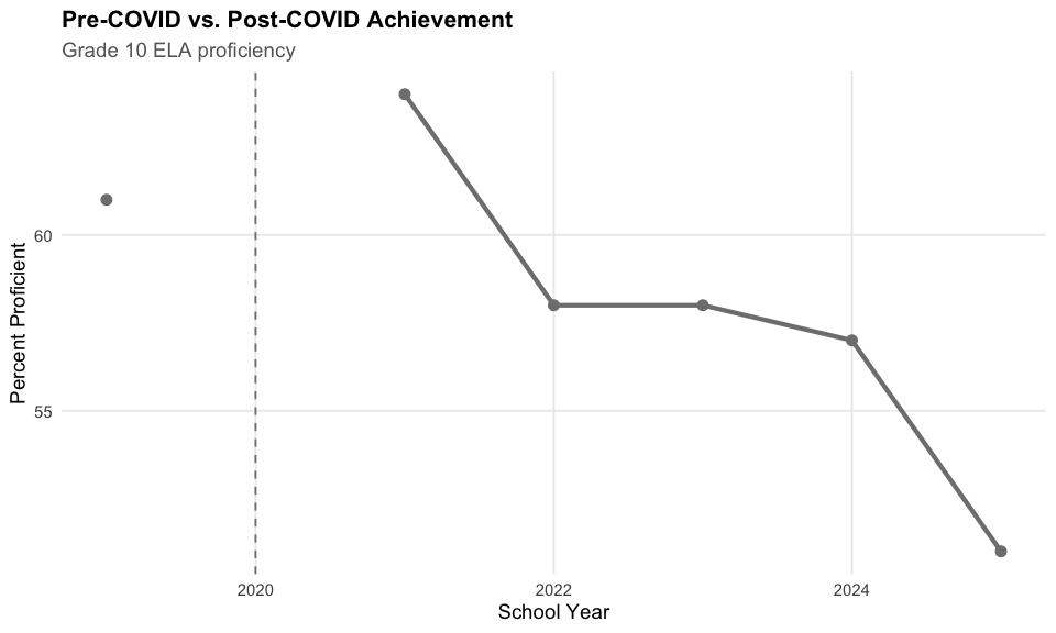
Data Notes
MCAS Assessment Data
- Source: Massachusetts DESE via Socrata API (educationtocareer.data.mass.gov)
- Dataset ID: i9w6-niyt (MCAS Achievement Results)
- Years Available: 2017-2019, 2021-2025 (no 2020 due to COVID pandemic)
Proficiency Levels
MCAS uses four performance levels: - Exceeding Expectations (E): Advanced understanding - Meeting Expectations (M): Grade-level proficiency - Partially Meeting Expectations (PM): Approaching proficiency - Not Meeting Expectations (NM): Below grade level
“Meeting or Exceeding” (M+E) is the standard proficiency benchmark.
Suppression Rules
- Data suppressed when N < 10 students to protect privacy
- Percentages may not sum to 100% due to rounding
Grade Levels Tested
- Grades 3-8: ELA and Math annually
- Grade 5 & 8: Science
- Grade 10: ELA, Math, and Science (high school graduation requirement)
- High School Science: Biology or Physics
sessionInfo()
#> R version 4.5.2 (2025-10-31)
#> Platform: x86_64-pc-linux-gnu
#> Running under: Ubuntu 24.04.3 LTS
#>
#> Matrix products: default
#> BLAS:   /usr/lib/x86_64-linux-gnu/openblas-pthread/libblas.so.3
#> LAPACK: /usr/lib/x86_64-linux-gnu/openblas-pthread/libopenblasp-r0.3.26.so;  LAPACK version 3.12.0
#>
#> locale:
#>  [1] LC_CTYPE=C.UTF-8       LC_NUMERIC=C           LC_TIME=C.UTF-8
#>  [4] LC_COLLATE=C.UTF-8     LC_MONETARY=C.UTF-8    LC_MESSAGES=C.UTF-8
#>  [7] LC_PAPER=C.UTF-8       LC_NAME=C              LC_ADDRESS=C
#> [10] LC_TELEPHONE=C         LC_MEASUREMENT=C.UTF-8 LC_IDENTIFICATION=C
#>
#> time zone: UTC
#> tzcode source: system (glibc)
#>
#> attached base packages:
#> [1] stats     graphics  grDevices utils     datasets  methods   base
#>
#> other attached packages:
#> [1] scales_1.4.0       dplyr_1.2.0        ggplot2_4.0.2      maschooldata_0.1.0
#>
#> loaded via a namespace (and not attached):
#>  [1] gtable_0.3.6       jsonlite_2.0.0     compiler_4.5.2     tidyselect_1.2.1
#>  [5] tidyr_1.3.2        jquerylib_0.1.4    systemfonts_1.3.2  textshaping_1.0.5
#>  [9] yaml_2.3.12        fastmap_1.2.0      R6_2.6.1           labeling_0.4.3
#> [13] generics_0.1.4     curl_7.0.0         knitr_1.51         tibble_3.3.1
#> [17] desc_1.4.3         bslib_0.10.0       pillar_1.11.1      RColorBrewer_1.1-3
#> [21] rlang_1.1.7        utf8_1.2.6         cachem_1.1.0       xfun_0.56
#> [25] fs_1.6.7           sass_0.4.10        S7_0.2.1           cli_3.6.5
#> [29] pkgdown_2.2.0      withr_3.0.2        magrittr_2.0.4     digest_0.6.39
#> [33] grid_4.5.2         rappdirs_0.3.4     lifecycle_1.0.5    vctrs_0.7.1
#> [37] evaluate_1.0.5     glue_1.8.0         farver_2.1.2       codetools_0.2-20
#> [41] ragg_1.5.1         httr_1.4.8         rmarkdown_2.30     purrr_1.2.1
#> [45] tools_4.5.2        pkgconfig_2.0.3    htmltools_0.5.9