library(nmschooldata)
library(dplyr)
library(tidyr)
library(ggplot2)

theme_set(theme_minimal(base_size = 14))
New Mexico – the Land of Enchantment – enrolls about 307,000 students across 155 districts and 876 schools. This vignette explores 10 years of enrollment data (2016-2025) from the New Mexico Public Education Department, surfacing 15 data stories hiding in the numbers.
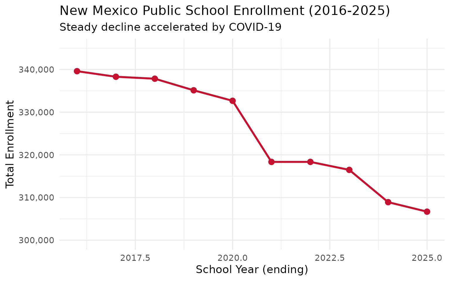
1. New Mexico lost 33,000 students in a decade
From 2016 to 2025, statewide enrollment fell from 340,000 to 307,000 – a 9.7% decline that accelerated dramatically during the pandemic year of 2021.
all_years <- fetch_enr_multi(2016:2025, use_cache = TRUE)

state_totals <- all_years |>
  filter(is_state, subgroup == "total_enrollment", grade_level == "TOTAL") |>
  select(end_year, n_students) |>
  mutate(change = n_students - lag(n_students),
         pct_change = round(change / lag(n_students) * 100, 2))

stopifnot(nrow(state_totals) > 0)
state_totals
#>    end_year n_students change pct_change
#> 1      2016     339613     NA         NA
#> 2      2017     338307  -1306      -0.38
#> 3      2018     337847   -460      -0.14
#> 4      2019     335131  -2716      -0.80
#> 5      2020     332672  -2459      -0.73
#> 6      2021     318349 -14323      -4.31
#> 7      2022     318353      4       0.00
#> 8      2023     316478  -1875      -0.59
#> 9      2024     308913  -7565      -2.39
#> 10     2025     306686  -2227      -0.72
ggplot(state_totals, aes(x = end_year, y = n_students)) +
  geom_line(linewidth = 1.2, color = "#C41230") +
  geom_point(size = 3, color = "#C41230") +
  scale_y_continuous(labels = scales::comma, limits = c(300000, 345000)) +
  labs(
    title = "New Mexico Public School Enrollment (2016-2025)",
    subtitle = "Steady decline accelerated by COVID-19",
    x = "School Year (ending)",
    y = "Total Enrollment"
  )
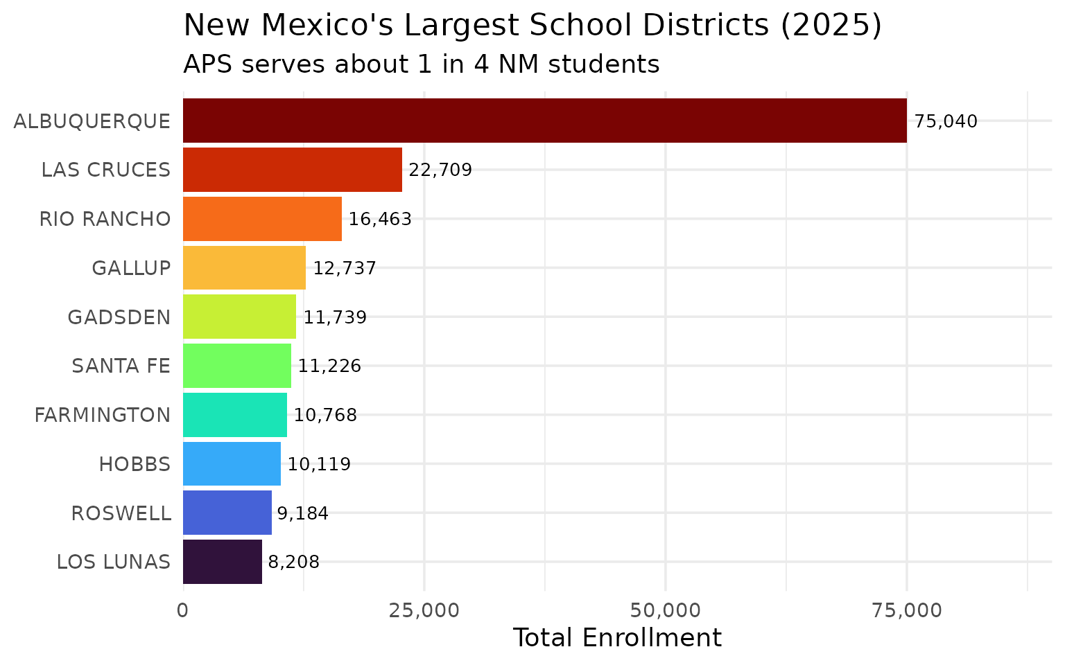
2. Albuquerque enrolls 1 in 4 NM students but is shrinking fastest
Albuquerque Public Schools is a colossus – 75,000 students, nearly 25% of the entire state. But APS lost 17,000 students since 2016, a decline steeper than the state average.
enr_2025 <- fetch_enr(2025, use_cache = TRUE)

top_districts <- enr_2025 |>
  filter(is_district, subgroup == "total_enrollment", grade_level == "TOTAL") |>
  arrange(desc(n_students)) |>
  head(10) |>
  select(district_name, n_students)

stopifnot(nrow(top_districts) > 0)
top_districts
#>    district_name n_students
#> 1    ALBUQUERQUE      75040
#> 2     LAS CRUCES      22709
#> 3     RIO RANCHO      16463
#> 4         GALLUP      12737
#> 5        GADSDEN      11739
#> 6       SANTA FE      11226
#> 7     FARMINGTON      10768
#> 8          HOBBS      10119
#> 9        ROSWELL       9184
#> 10     LOS LUNAS       8208
top_districts |>
  mutate(district_name = forcats::fct_reorder(district_name, n_students)) |>
  ggplot(aes(x = n_students, y = district_name, fill = district_name)) +
  geom_col(show.legend = FALSE) +
  geom_text(aes(label = scales::comma(n_students)), hjust = -0.1, size = 3.5) +
  scale_x_continuous(labels = scales::comma, expand = expansion(mult = c(0, 0.2))) +
  scale_fill_viridis_d(option = "turbo") +
  labs(
    title = "New Mexico's Largest School Districts (2025)",
    subtitle = "APS serves about 1 in 4 NM students",
    x = "Total Enrollment",
    y = NULL
  )
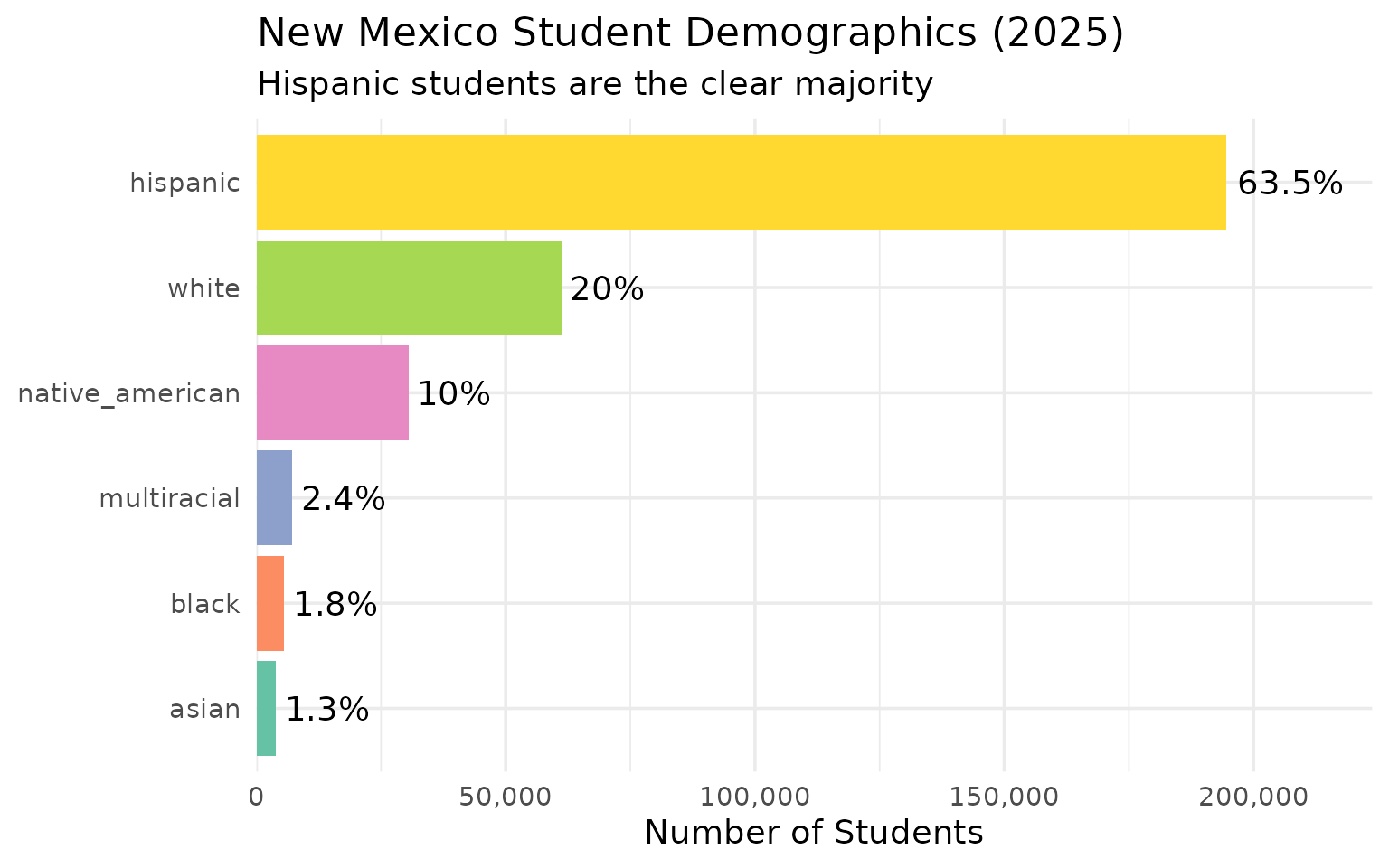
3. Hispanic students are 63% of enrollment – and the share keeps rising
New Mexico is one of only two majority-Hispanic states in the country. The Hispanic share of enrollment has grown from 61.8% in 2019 to 63.5% in 2025 even as overall enrollment shrinks.
Data caveat: In 2025, NM PED began reporting multiracial students as a separate category (7,221 students, previously 0). Some apparent declines in other race/ethnicity groups between 2023 and 2025 are partly reclassification effects, not actual population changes.
demographics <- enr_2025 |>
  filter(is_state, grade_level == "TOTAL",
         subgroup %in% c("hispanic", "white", "native_american", "black", "asian", "multiracial")) |>
  mutate(pct = round(pct * 100, 1)) |>
  select(subgroup, n_students, pct) |>
  arrange(desc(n_students))

stopifnot(nrow(demographics) > 0)
demographics
#>          subgroup n_students  pct
#> 1        hispanic     194595 63.5
#> 2           white      61345 20.0
#> 3 native_american      30602 10.0
#> 4     multiracial       7221  2.4
#> 5           black       5580  1.8
#> 6           asian       3926  1.3
demographics |>
  mutate(subgroup = forcats::fct_reorder(subgroup, n_students)) |>
  ggplot(aes(x = n_students, y = subgroup, fill = subgroup)) +
  geom_col(show.legend = FALSE) +
  geom_text(aes(label = paste0(pct, "%")), hjust = -0.1) +
  scale_x_continuous(labels = scales::comma, expand = expansion(mult = c(0, 0.15))) +
  scale_fill_brewer(palette = "Set2") +
  labs(
    title = "New Mexico Student Demographics (2025)",
    subtitle = "Hispanic students are the clear majority",
    x = "Number of Students",
    y = NULL
  )
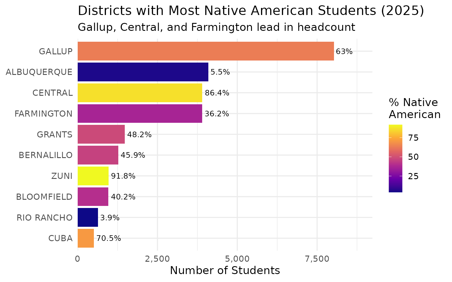
4. Gallup leads the state in Native American enrollment
New Mexico has the third-highest Native American student population in the country, concentrated in districts near the Navajo Nation, Zuni, and numerous Pueblos. Gallup alone enrolls over 8,000 Native American students.
native_am <- enr_2025 |>
  filter(is_district, subgroup == "native_american", grade_level == "TOTAL") |>
  arrange(desc(n_students)) |>
  head(10) |>
  select(district_name, n_students, pct) |>
  mutate(pct = round(pct * 100, 1))

stopifnot(nrow(native_am) > 0)
native_am
#>    district_name n_students  pct
#> 1         GALLUP       8027 63.0
#> 2    ALBUQUERQUE       4093  5.5
#> 3        CENTRAL       3903 86.4
#> 4     FARMINGTON       3896 36.2
#> 5         GRANTS       1472 48.2
#> 6     BERNALILLO       1272 45.9
#> 7           ZUNI        966 91.8
#> 8     BLOOMFIELD        961 40.2
#> 9     RIO RANCHO        637  3.9
#> 10          CUBA        508 70.5
native_am |>
  mutate(district_name = forcats::fct_reorder(district_name, n_students)) |>
  ggplot(aes(x = n_students, y = district_name, fill = pct)) +
  geom_col() +
  geom_text(aes(label = paste0(pct, "%")), hjust = -0.1, size = 3.5) +
  scale_x_continuous(labels = scales::comma, expand = expansion(mult = c(0, 0.15))) +
  scale_fill_viridis_c(option = "plasma", name = "% Native\nAmerican") +
  labs(
    title = "Districts with Most Native American Students (2025)",
    subtitle = "Gallup, Central, and Farmington lead in headcount",
    x = "Number of Students",
    y = NULL
  )
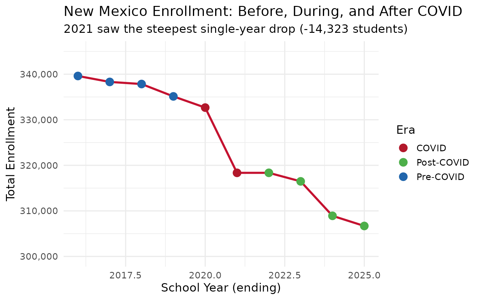
5. COVID wiped out 14,000 students in a single year
The 2021 school year (2020-21) saw a staggering 4.3% enrollment drop – 14,323 students vanished from NM classrooms. Enrollment has never recovered.
covid_era <- all_years |>
  filter(is_state, subgroup == "total_enrollment", grade_level == "TOTAL",
         end_year %in% c(2019, 2020, 2021, 2022, 2023)) |>
  select(end_year, n_students) |>
  mutate(change = n_students - lag(n_students),
         pct_change = round(change / lag(n_students) * 100, 2))

stopifnot(nrow(covid_era) > 0)
covid_era
#>   end_year n_students change pct_change
#> 1     2019     335131     NA         NA
#> 2     2020     332672  -2459      -0.73
#> 3     2021     318349 -14323      -4.31
#> 4     2022     318353      4       0.00
#> 5     2023     316478  -1875      -0.59
decline_data <- all_years |>
  filter(is_state, subgroup == "total_enrollment", grade_level == "TOTAL") |>
  mutate(era = case_when(
    end_year <= 2019 ~ "Pre-COVID",
    end_year <= 2021 ~ "COVID",
    TRUE ~ "Post-COVID"
  ))

stopifnot(nrow(decline_data) > 0)

decline_data |>
  ggplot(aes(x = end_year, y = n_students, color = era)) +
  geom_line(linewidth = 1.2, color = "#C41230") +
  geom_point(aes(color = era), size = 4) +
  scale_y_continuous(labels = scales::comma, limits = c(300000, 345000)) +
  scale_color_manual(values = c("Pre-COVID" = "#2166AC", "COVID" = "#B2182B", "Post-COVID" = "#4DAF4A")) +
  labs(
    title = "New Mexico Enrollment: Before, During, and After COVID",
    subtitle = "2021 saw the steepest single-year drop (-14,323 students)",
    x = "School Year (ending)",
    y = "Total Enrollment",
    color = "Era"
  )
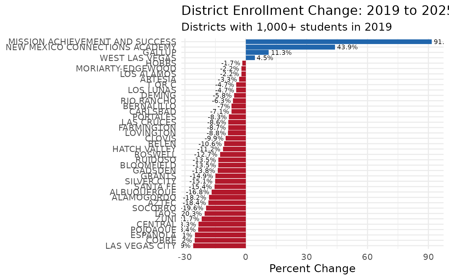
6. Albuquerque lost 17,000 students while Gallup grew 11%
Not all districts are declining. Gallup gained 1,289 students (+11.3%) from 2019 to 2025, while Albuquerque hemorrhaged over 15,000. The divergence reveals a stark urban-rural-tribal split.
enr_2019 <- fetch_enr(2019, use_cache = TRUE)

d_2019 <- enr_2019 |>
  filter(is_school, subgroup == "total_enrollment", grade_level == "TOTAL") |>
  group_by(district_name) |>
  summarize(n_2019 = sum(n_students))

d_2025 <- enr_2025 |>
  filter(is_district, subgroup == "total_enrollment", grade_level == "TOTAL") |>
  select(district_name, n_2025 = n_students)

growth <- inner_join(d_2019, d_2025, by = "district_name") |>
  mutate(change = n_2025 - n_2019,
         pct_change = round((n_2025 / n_2019 - 1) * 100, 1)) |>
  filter(n_2019 >= 1000) |>
  arrange(pct_change)

stopifnot(nrow(growth) > 0)
growth |> select(district_name, n_2019, n_2025, pct_change)
#> # A tibble: 39 × 4
#>    district_name  n_2019 n_2025 pct_change
#>    <chr>           <dbl>  <dbl>      <dbl>
#>  1 LAS VEGAS CITY   1512   1121      -25.9
#>  2 COBRE            1255    939      -25.2
#>  3 ESPANOLA         3555   2664      -25.1
#>  4 POJOAQUE         1965   1506      -23.4
#>  5 CENTRAL          5893   4519      -23.3
#>  6 ZUNI             1343   1052      -21.7
#>  7 TAOS             2741   2184      -20.3
#>  8 SOCORRO          1654   1329      -19.6
#>  9 AZTEC            3002   2449      -18.4
#> 10 ALAMOGORDO       6396   5229      -18.2
#> # ℹ 29 more rows
growth |>
  mutate(district_name = forcats::fct_reorder(district_name, pct_change)) |>
  ggplot(aes(x = pct_change, y = district_name, fill = pct_change > 0)) +
  geom_col(show.legend = FALSE) +
  geom_text(aes(label = paste0(pct_change, "%")),
            hjust = ifelse(growth$pct_change > 0, -0.1, 1.1), size = 3) +
  scale_fill_manual(values = c("TRUE" = "#2166AC", "FALSE" = "#B2182B")) +
  labs(
    title = "District Enrollment Change: 2019 to 2025",
    subtitle = "Districts with 1,000+ students in 2019",
    x = "Percent Change",
    y = NULL
  )
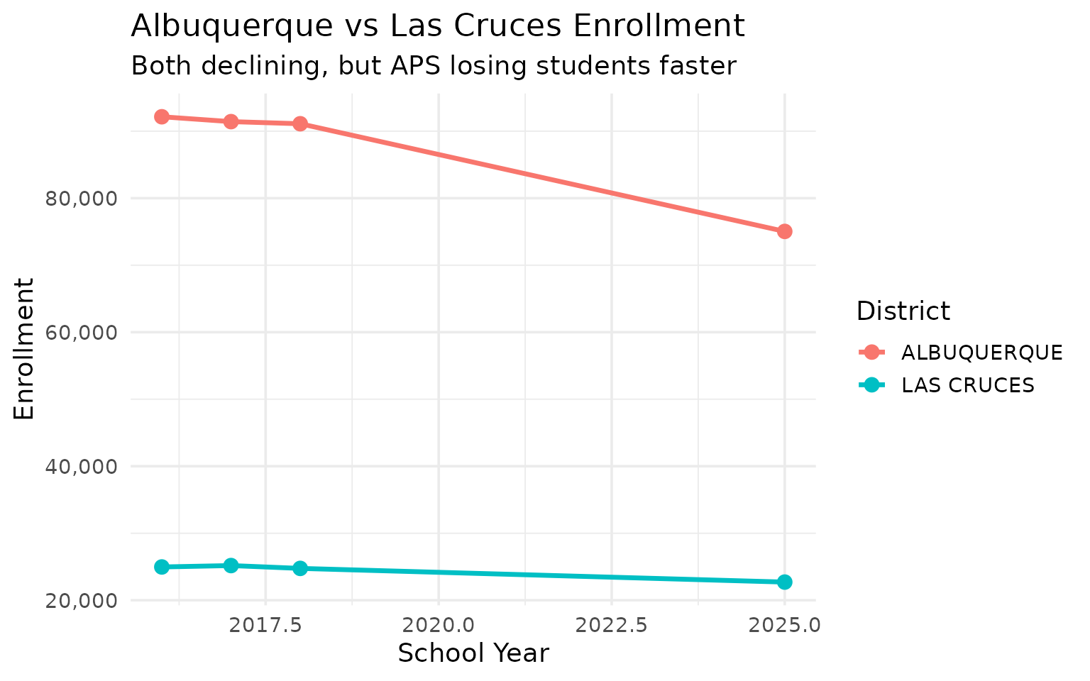
7. Albuquerque vs Las Cruces: Two cities, one direction
New Mexico’s two largest districts both lost students from 2016 to 2025, but Albuquerque’s decline (-18.6%) far outpaced Las Cruces (-9.0%).
enr_era1 <- fetch_enr_multi(2016:2018, use_cache = TRUE)

abq_lc_era1 <- enr_era1 |>
  filter(is_district, subgroup == "total_enrollment", grade_level == "TOTAL",
         district_name %in% c("ALBUQUERQUE", "LAS CRUCES")) |>
  select(end_year, district_name, n_students)

abq_lc_2025 <- enr_2025 |>
  filter(is_district, subgroup == "total_enrollment", grade_level == "TOTAL",
         district_name %in% c("ALBUQUERQUE", "LAS CRUCES")) |>
  select(end_year, district_name, n_students)

abq_lc <- bind_rows(abq_lc_era1, abq_lc_2025)
stopifnot(nrow(abq_lc) > 0)
abq_lc |> pivot_wider(names_from = end_year, values_from = n_students)
#> # A tibble: 2 × 5
#>   district_name `2016` `2017` `2018` `2025`
#>   <chr>          <dbl>  <dbl>  <dbl>  <dbl>
#> 1 ALBUQUERQUE    92152  91426  91110  75040
#> 2 LAS CRUCES     24965  25174  24751  22709
abq_lc |>
  ggplot(aes(x = end_year, y = n_students, color = district_name)) +
  geom_line(linewidth = 1.2) +
  geom_point(size = 3) +
  scale_y_continuous(labels = scales::comma) +
  labs(
    title = "Albuquerque vs Las Cruces Enrollment",
    subtitle = "Both declining, but APS losing students faster",
    x = "School Year",
    y = "Enrollment",
    color = "District"
  )
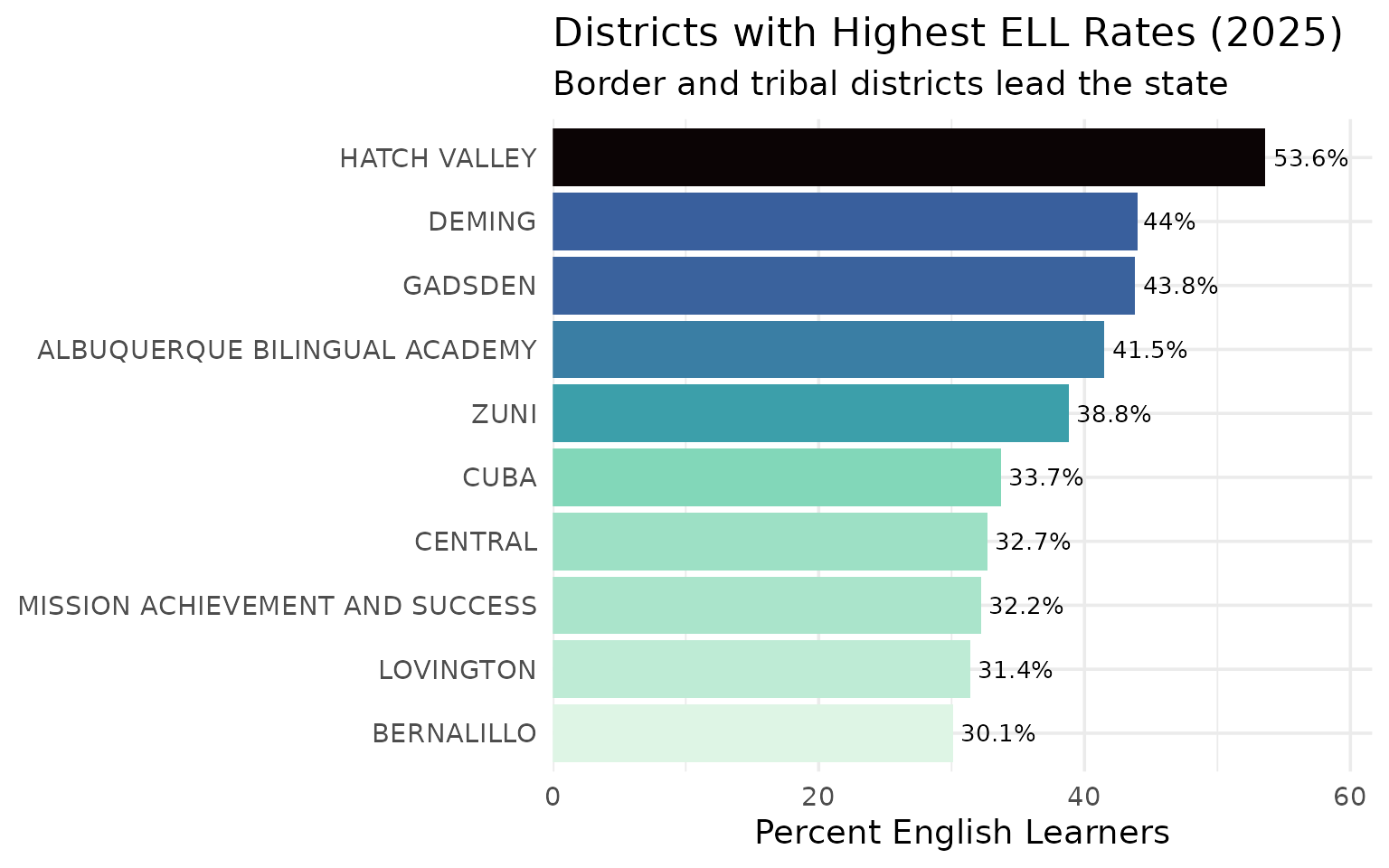
8. 1 in 5 NM students is an English Learner
New Mexico’s ELL rate of 18.2% is among the highest in the nation – more than double the national average. Border districts like Gadsden (43.8%) and Deming (44.0%) have the highest rates.
ell_trend <- all_years |>
  filter(is_state, subgroup == "ell", grade_level == "TOTAL") |>
  mutate(pct = round(pct * 100, 1)) |>
  select(end_year, n_students, pct)

stopifnot(nrow(ell_trend) > 0)
ell_trend
#>   end_year n_students  pct
#> 1     2019      50952 15.2
#> 2     2020      52719 15.8
#> 3     2021      49320 15.5
#> 4     2022      53572 16.8
#> 5     2023      55715 17.6
#> 6     2025      55798 18.2
ell_districts <- enr_2025 |>
  filter(is_district, subgroup == "ell", grade_level == "TOTAL",
         n_students >= 100) |>
  arrange(desc(pct)) |>
  head(10) |>
  select(district_name, n_students, pct) |>
  mutate(pct = round(pct * 100, 1))

stopifnot(nrow(ell_districts) > 0)
ell_districts
#>                      district_name n_students  pct
#> 1                     HATCH VALLEY        614 53.6
#> 2                           DEMING       2251 44.0
#> 3                          GADSDEN       5139 43.8
#> 4    ALBUQUERQUE BILINGUAL ACADEMY        136 41.5
#> 5                             ZUNI        408 38.8
#> 6                             CUBA        243 33.7
#> 7                          CENTRAL       1478 32.7
#> 8  MISSION ACHIEVEMENT AND SUCCESS        719 32.2
#> 9                        LOVINGTON       1071 31.4
#> 10                      BERNALILLO        836 30.1
ell_districts |>
  mutate(district_name = forcats::fct_reorder(district_name, pct)) |>
  ggplot(aes(x = pct, y = district_name, fill = pct)) +
  geom_col(show.legend = FALSE) +
  geom_text(aes(label = paste0(pct, "%")), hjust = -0.1, size = 3.5) +
  scale_x_continuous(expand = expansion(mult = c(0, 0.15))) +
  scale_fill_viridis_c(option = "mako", direction = -1) +
  labs(
    title = "Districts with Highest ELL Rates (2025)",
    subtitle = "Border and tribal districts lead the state",
    x = "Percent English Learners",
    y = NULL
  )
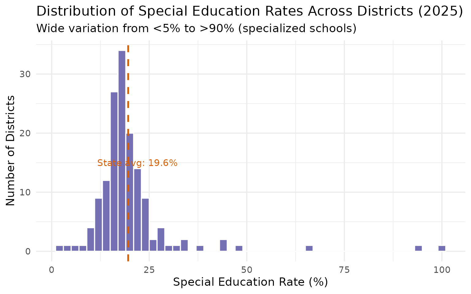
9. Special education enrollment is surging
The special education rate climbed from 15.9% in 2019 to 19.6% in 2025 – an increase of nearly 7,000 students even as total enrollment fell. Nearly 1 in 5 NM students now receives special education services.
sped_trend <- all_years |>
  filter(is_state, subgroup == "special_ed", grade_level == "TOTAL") |>
  mutate(pct = round(pct * 100, 1)) |>
  select(end_year, n_students, pct)

stopifnot(nrow(sped_trend) > 0)
sped_trend
#>   end_year n_students  pct
#> 1     2019      53253 15.9
#> 2     2020      55070 16.6
#> 3     2021      53477 16.8
#> 4     2022      53762 16.9
#> 5     2023      55537 17.5
#> 6     2025      60257 19.6
sped_districts <- enr_2025 |>
  filter(is_district, subgroup == "special_ed", grade_level == "TOTAL") |>
  mutate(pct = round(pct * 100, 1))

stopifnot(nrow(sped_districts) > 0)

ggplot(sped_districts, aes(x = pct)) +
  geom_histogram(binwidth = 2, fill = "#7570B3", color = "white") +
  geom_vline(xintercept = 19.6, linetype = "dashed", color = "#D95F02", linewidth = 1) +
  annotate("text", x = 22, y = 15, label = "State avg: 19.6%", color = "#D95F02", size = 4) +
  labs(
    title = "Distribution of Special Education Rates Across Districts (2025)",
    subtitle = "Wide variation from <5% to >90% (specialized schools)",
    x = "Special Education Rate (%)",
    y = "Number of Districts"
  )
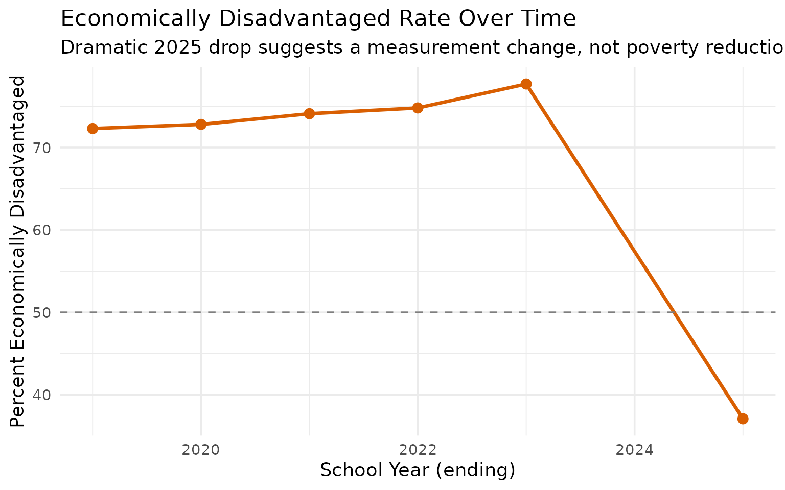
10. 72% of NM students were economically disadvantaged – until 2025
New Mexico’s economically disadvantaged rate hovered around 72-78% from 2019-2023, then plummeted to 37.1% in 2025. The dramatic drop likely reflects a change in how NM PED measures economic disadvantage, not an actual improvement in child poverty.
ed_trend <- all_years |>
  filter(is_state, subgroup == "econ_disadv", grade_level == "TOTAL") |>
  mutate(pct = round(pct * 100, 1)) |>
  select(end_year, n_students, pct)

stopifnot(nrow(ed_trend) > 0)
ed_trend
#>   end_year n_students  pct
#> 1     2019     242160 72.3
#> 2     2020     242159 72.8
#> 3     2021     236008 74.1
#> 4     2022     238033 74.8
#> 5     2023     245845 77.7
#> 6     2025     113772 37.1
ed_trend |>
  ggplot(aes(x = end_year, y = pct)) +
  geom_line(linewidth = 1.2, color = "#D95F02") +
  geom_point(size = 3, color = "#D95F02") +
  geom_hline(yintercept = 50, linetype = "dashed", color = "gray50") +
  labs(
    title = "Economically Disadvantaged Rate Over Time",
    subtitle = "Dramatic 2025 drop suggests a measurement change, not poverty reduction",
    x = "School Year (ending)",
    y = "Percent Economically Disadvantaged"
  )
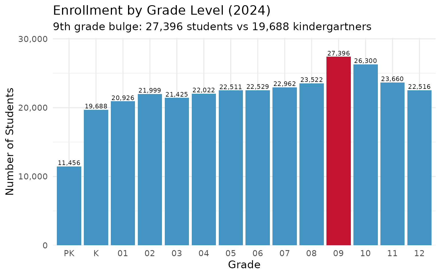
11. 9th grade is the biggest grade – a demographic bulge
New Mexico’s 9th grade consistently has thousands more students than any other grade. In 2024, 9th grade had 27,396 students versus just 19,688 in kindergarten – a 39% gap that signals both grade retention and rising dropout risk.
enr_2024 <- fetch_enr(2024, use_cache = TRUE)

grade_data <- enr_2024 |>
  filter(is_state, subgroup == "total_enrollment",
         grade_level %in% c("PK", "K", "01", "02", "03", "04", "05",
                            "06", "07", "08", "09", "10", "11", "12")) |>
  select(grade_level, n_students) |>
  mutate(grade_level = factor(grade_level,
    levels = c("PK", "K", "01", "02", "03", "04", "05",
               "06", "07", "08", "09", "10", "11", "12")))

stopifnot(nrow(grade_data) > 0)
grade_data
#>    grade_level n_students
#> 1           PK      11456
#> 2            K      19688
#> 3           01      20926
#> 4           02      21999
#> 5           03      21425
#> 6           04      22022
#> 7           05      22511
#> 8           06      22529
#> 9           07      22962
#> 10          08      23522
#> 11          09      27396
#> 12          10      26300
#> 13          11      23660
#> 14          12      22516
ggplot(grade_data, aes(x = grade_level, y = n_students, fill = grade_level == "09")) +
  geom_col(show.legend = FALSE) +
  geom_text(aes(label = scales::comma(n_students)), vjust = -0.3, size = 3) +
  scale_fill_manual(values = c("TRUE" = "#C41230", "FALSE" = "#4393C3")) +
  scale_y_continuous(labels = scales::comma, expand = expansion(mult = c(0, 0.1))) +
  labs(
    title = "Enrollment by Grade Level (2024)",
    subtitle = "9th grade bulge: 27,396 students vs 19,688 kindergartners",
    x = "Grade",
    y = "Number of Students"
  )
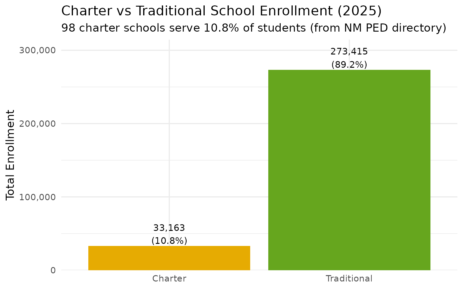
12. Charter schools enroll 10.8% of students across 98 schools
New Mexico has 98 charter schools enrolling 33,163 students – 10.8%
of statewide enrollment. The charter sector includes 58 state-chartered
schools (authorized by the Public Education Commission, operating as
their own LEA) and 42 locally-authorized charters within traditional
districts (30 under APS alone). The is_charter flag is
derived from NM PED’s official school directory, not name-pattern
matching.
charters <- enr_2025 |>
  filter(is_school, subgroup == "total_enrollment", grade_level == "TOTAL") |>
  group_by(is_charter) |>
  summarize(
    n_schools = n(),
    total_enrollment = sum(n_students),
    .groups = "drop"
  ) |>
  mutate(pct_enrollment = round(total_enrollment / sum(total_enrollment) * 100, 1))

stopifnot(nrow(charters) > 0)
charters
#> # A tibble: 2 × 4
#>   is_charter n_schools total_enrollment pct_enrollment
#>   <lgl>          <int>            <dbl>          <dbl>
#> 1 FALSE            778           273415           89.2
#> 2 TRUE              98            33163           10.8
charters |>
  mutate(label = ifelse(is_charter, "Charter", "Traditional")) |>
  ggplot(aes(x = label, y = total_enrollment, fill = label)) +
  geom_col(show.legend = FALSE) +
  geom_text(aes(label = paste0(scales::comma(total_enrollment), "\n(",
                                pct_enrollment, "%)")),
            vjust = -0.1, size = 4) +
  scale_y_continuous(labels = scales::comma, expand = expansion(mult = c(0, 0.15))) +
  scale_fill_manual(values = c("Charter" = "#E6AB02", "Traditional" = "#66A61E")) +
  labs(
    title = "Charter vs Traditional School Enrollment (2025)",
    subtitle = "98 charter schools serve 10.8% of students (from NM PED directory)",
    x = NULL,
    y = "Total Enrollment"
  )
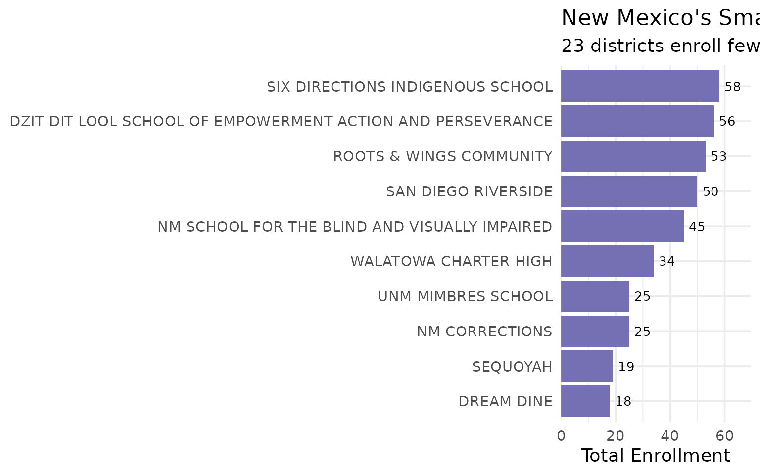
13. The smallest districts: 18 students in Dream Dine
New Mexico has 23 districts with fewer than 100 students. The smallest – Dream Dine – serves just 18 students. These tiny districts are disproportionately tribal and charter schools operating in remote communities.
smallest <- enr_2025 |>
  filter(is_district, subgroup == "total_enrollment", grade_level == "TOTAL") |>
  arrange(n_students) |>
  head(10) |>
  select(district_name, n_students)

stopifnot(nrow(smallest) > 0)
smallest
#>                                                  district_name n_students
#> 1                                                   DREAM DINE         18
#> 2                                                     SEQUOYAH         19
#> 3                                               NM CORRECTIONS         25
#> 4                                           UNM MIMBRES SCHOOL         25
#> 5                                        WALATOWA CHARTER HIGH         34
#> 6                NM SCHOOL FOR THE BLIND AND VISUALLY IMPAIRED         45
#> 7                                          SAN DIEGO RIVERSIDE         50
#> 8                                      ROOTS & WINGS COMMUNITY         53
#> 9  DZIT DIT LOOL SCHOOL OF EMPOWERMENT ACTION AND PERSEVERANCE         56
#> 10                            SIX DIRECTIONS INDIGENOUS SCHOOL         58
smallest |>
  mutate(district_name = forcats::fct_reorder(district_name, n_students)) |>
  ggplot(aes(x = n_students, y = district_name)) +
  geom_col(fill = "#7570B3") +
  geom_text(aes(label = n_students), hjust = -0.3, size = 3.5) +
  scale_x_continuous(expand = expansion(mult = c(0, 0.2))) +
  labs(
    title = "New Mexico's Smallest Districts (2025)",
    subtitle = "23 districts enroll fewer than 100 students",
    x = "Total Enrollment",
    y = NULL
  )
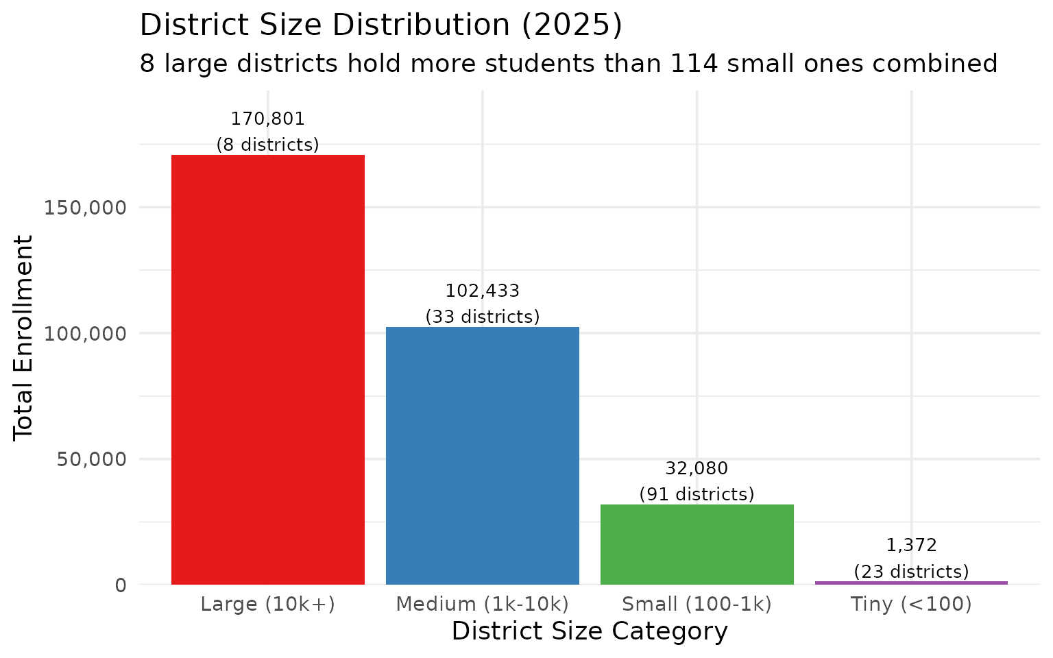
14. The rural-urban divide: 8 large districts hold 56% of students
Eight districts with 10,000+ students enroll 171,000 of the state’s 307,000 students. Meanwhile, 114 small and tiny districts share just 33,000 students between them.
size_dist <- enr_2025 |>
  filter(is_district, subgroup == "total_enrollment", grade_level == "TOTAL") |>
  mutate(size_category = case_when(
    n_students >= 10000 ~ "Large (10k+)",
    n_students >= 1000 ~ "Medium (1k-10k)",
    n_students >= 100 ~ "Small (100-1k)",
    TRUE ~ "Tiny (<100)"
  )) |>
  group_by(size_category) |>
  summarize(
    n_districts = n(),
    total_students = sum(n_students),
    .groups = "drop"
  ) |>
  mutate(size_category = factor(size_category,
    levels = c("Large (10k+)", "Medium (1k-10k)", "Small (100-1k)", "Tiny (<100)")))

stopifnot(nrow(size_dist) > 0)
size_dist
#> # A tibble: 4 × 3
#>   size_category   n_districts total_students
#>   <fct>                 <int>          <dbl>
#> 1 Large (10k+)              8         170801
#> 2 Medium (1k-10k)          33         102433
#> 3 Small (100-1k)           91          32080
#> 4 Tiny (<100)              23           1372
size_dist |>
  ggplot(aes(x = size_category, y = total_students, fill = size_category)) +
  geom_col(show.legend = FALSE) +
  geom_text(aes(label = paste0(scales::comma(total_students), "\n(",
                                n_districts, " districts)")),
            vjust = -0.1, size = 3.5) +
  scale_y_continuous(labels = scales::comma, expand = expansion(mult = c(0, 0.15))) +
  scale_fill_brewer(palette = "Set1") +
  labs(
    title = "District Size Distribution (2025)",
    subtitle = "8 large districts hold more students than 114 small ones combined",
    x = "District Size Category",
    y = "Total Enrollment"
  )
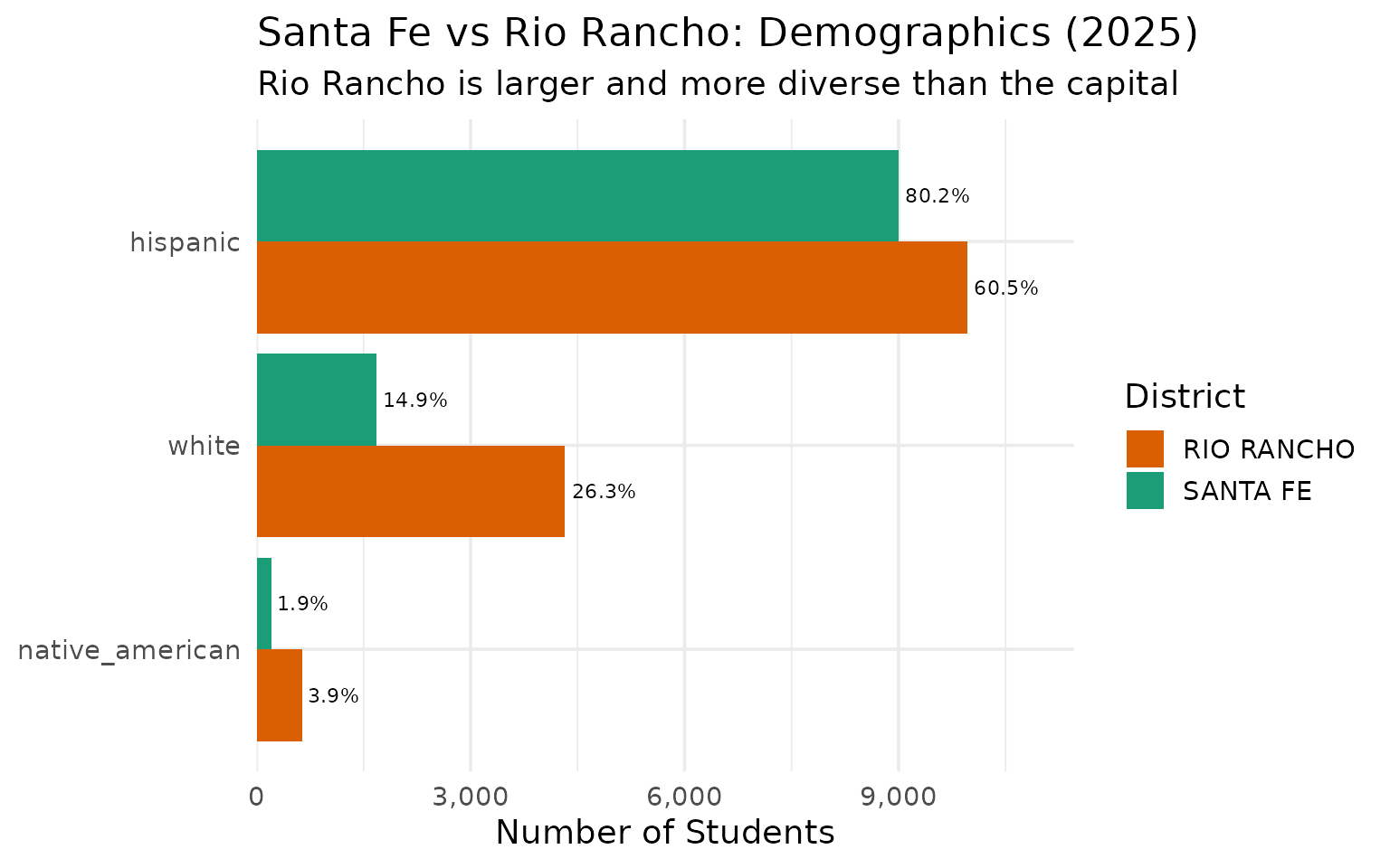
15. Santa Fe vs Rio Rancho: The capital falls behind the suburb
Rio Rancho – a fast-growing Albuquerque suburb – now enrolls 16,463 students, surpassing the state capital Santa Fe (11,226) by over 5,000 students. Rio Rancho has become NM’s third-largest district.
sf_rr <- enr_2025 |>
  filter(is_district, subgroup %in% c("total_enrollment", "hispanic", "white", "native_american"),
         grade_level == "TOTAL",
         district_name %in% c("SANTA FE", "RIO RANCHO")) |>
  select(district_name, subgroup, n_students, pct) |>
  mutate(pct = round(pct * 100, 1))

stopifnot(nrow(sf_rr) > 0)
sf_rr |> pivot_wider(names_from = subgroup, values_from = c(n_students, pct))
#> # A tibble: 2 × 9
#>   district_name n_students_total_enrollment n_students_white n_students_hispanic
#>   <chr>                               <dbl>            <dbl>               <dbl>
#> 1 RIO RANCHO                          16463             4324                9963
#> 2 SANTA FE                            11226             1676                8999
#> # ℹ 5 more variables: n_students_native_american <dbl>,
#> #   pct_total_enrollment <dbl>, pct_white <dbl>, pct_hispanic <dbl>,
#> #   pct_native_american <dbl>
sf_rr |>
  filter(subgroup != "total_enrollment") |>
  mutate(subgroup = forcats::fct_reorder(subgroup, n_students)) |>
  ggplot(aes(x = n_students, y = subgroup, fill = district_name)) +
  geom_col(position = "dodge") +
  geom_text(aes(label = paste0(pct, "%")), position = position_dodge(0.9),
            hjust = -0.1, size = 3) +
  scale_x_continuous(labels = scales::comma, expand = expansion(mult = c(0, 0.15))) +
  scale_fill_manual(values = c("SANTA FE" = "#1B9E77", "RIO RANCHO" = "#D95F02")) +
  labs(
    title = "Santa Fe vs Rio Rancho: Demographics (2025)",
    subtitle = "Rio Rancho is larger and more diverse than the capital",
    x = "Number of Students",
    y = NULL,
    fill = "District"
  )
Summary
New Mexico’s school enrollment data reveals:
- Declining enrollment: The state lost 33,000 students from 2016 to 2025
- Hispanic majority: 63.5% of students are Hispanic, and the share is growing
- Native American presence: Third-highest tribal enrollment in the nation
- Urban concentration: APS serves 1 in 4 students statewide
- COVID impact: 14,000 students lost in a single year (2021), never recovered
- ELL surge: 18.2% English Learner rate, more than double the national average
- SPED growth: Special education climbed from 15.9% to 19.6% in six years
- Charter presence: 98 charter schools serve 10.8% of students
- Rural fragmentation: 114 districts serve fewer than 1,000 students each
These patterns shape school funding debates and facility planning across the Land of Enchantment.
Data sourced from the New Mexico Public Education Department STARS System.
sessionInfo()
#> R version 4.5.2 (2025-10-31)
#> Platform: x86_64-pc-linux-gnu
#> Running under: Ubuntu 24.04.3 LTS
#>
#> Matrix products: default
#> BLAS:   /usr/lib/x86_64-linux-gnu/openblas-pthread/libblas.so.3
#> LAPACK: /usr/lib/x86_64-linux-gnu/openblas-pthread/libopenblasp-r0.3.26.so;  LAPACK version 3.12.0
#>
#> locale:
#>  [1] LC_CTYPE=C.UTF-8       LC_NUMERIC=C           LC_TIME=C.UTF-8
#>  [4] LC_COLLATE=C.UTF-8     LC_MONETARY=C.UTF-8    LC_MESSAGES=C.UTF-8
#>  [7] LC_PAPER=C.UTF-8       LC_NAME=C              LC_ADDRESS=C
#> [10] LC_TELEPHONE=C         LC_MEASUREMENT=C.UTF-8 LC_IDENTIFICATION=C
#>
#> time zone: UTC
#> tzcode source: system (glibc)
#>
#> attached base packages:
#> [1] stats     graphics  grDevices utils     datasets  methods   base
#>
#> other attached packages:
#> [1] ggplot2_4.0.2      tidyr_1.3.2        dplyr_1.2.0        nmschooldata_0.1.0
#>
#> loaded via a namespace (and not attached):
#>  [1] gtable_0.3.6       jsonlite_2.0.0     compiler_4.5.2     tidyselect_1.2.1
#>  [5] jquerylib_0.1.4    systemfonts_1.3.2  scales_1.4.0       textshaping_1.0.5
#>  [9] readxl_1.4.5       yaml_2.3.12        fastmap_1.2.0      R6_2.6.1
#> [13] labeling_0.4.3     generics_0.1.4     curl_7.0.0         knitr_1.51
#> [17] forcats_1.0.1      tibble_3.3.1       desc_1.4.3         bslib_0.10.0
#> [21] pillar_1.11.1      RColorBrewer_1.1-3 rlang_1.1.7        utf8_1.2.6
#> [25] cachem_1.1.0       xfun_0.56          S7_0.2.1           fs_1.6.7
#> [29] sass_0.4.10        viridisLite_0.4.3  cli_3.6.5          withr_3.0.2
#> [33] pkgdown_2.2.0      magrittr_2.0.4     digest_0.6.39      grid_4.5.2
#> [37] rappdirs_0.3.4     lifecycle_1.0.5    vctrs_0.7.1        evaluate_1.0.5
#> [41] glue_1.8.0         cellranger_1.1.0   farver_2.1.2       ragg_1.5.1
#> [45] httr_1.4.8         rmarkdown_2.30     purrr_1.2.1        tools_4.5.2
#> [49] pkgconfig_2.0.3    htmltools_0.5.9