15 Insights from Tennessee School Enrollment Data
Source:vignettes/enrollment_hooks.Rmd
enrollment_hooks.Rmd
library(tnschooldata)
library(dplyr)
library(tidyr)
library(ggplot2)
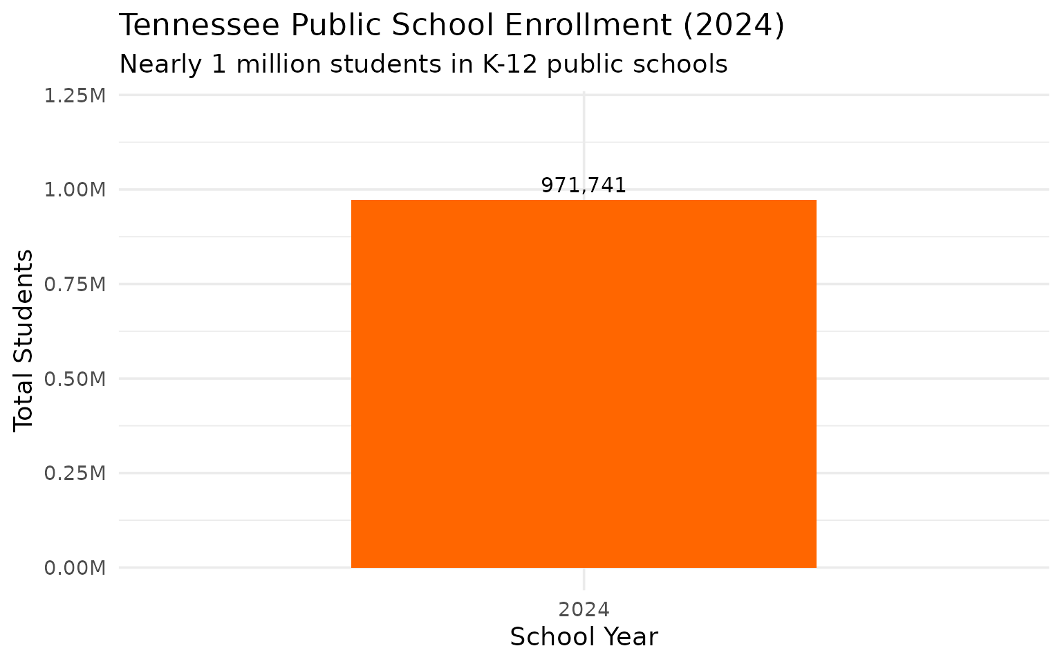
theme_set(theme_minimal(base_size = 14))1. Tennessee has nearly 1 million public school students
The Volunteer State serves a massive public school population, just shy of the million mark.
enr_2024 <- fetch_enr(2024, use_cache = TRUE)

statewide <- enr_2024 %>%
  filter(is_state, subgroup == "total_enrollment", grade_level == "TOTAL") %>%
  select(end_year, n_students)

stopifnot(nrow(statewide) > 0)
statewide
#>   end_year n_students
#> 1     2024     971741
statewide %>% print()
#>   end_year n_students
#> 1     2024     971741
ggplot(statewide, aes(x = factor(end_year), y = n_students / 1e6)) +
  geom_col(fill = "#FF6600", width = 0.6) +
  geom_text(aes(label = scales::comma(n_students)), vjust = -0.5, size = 4) +
  scale_y_continuous(
    labels = scales::label_number(suffix = "M"),
    limits = c(0, 1.2)
  ) +
  labs(
    title = "Tennessee Public School Enrollment (2024)",
    subtitle = "Nearly 1 million students in K-12 public schools",
    x = "School Year",
    y = "Total Students"
  )
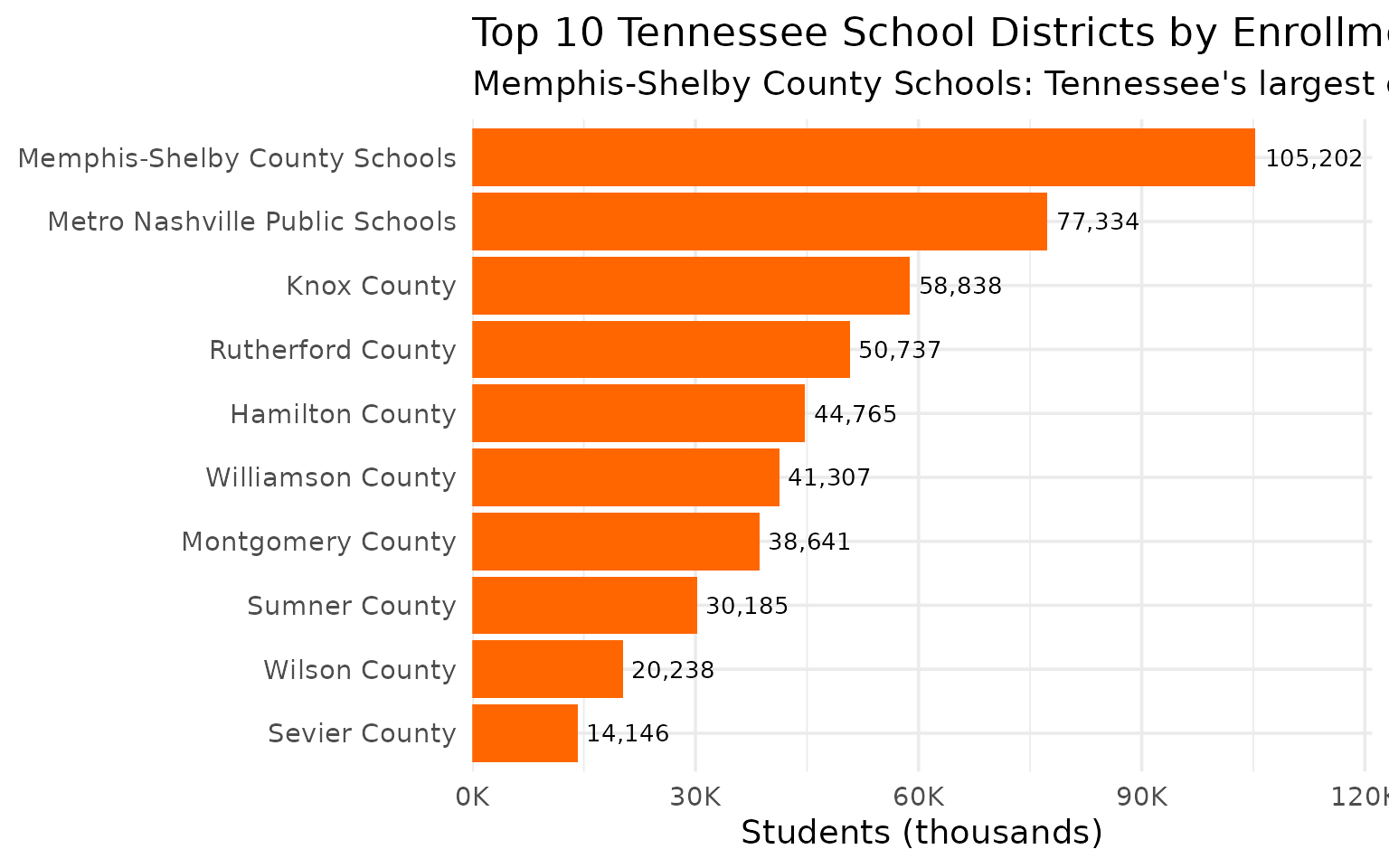
2. Memphis-Shelby County Schools dwarfs all other districts
Memphis’s merged district has more students than Nashville and Knoxville combined.
top_districts <- enr_2024 %>%
  filter(is_district, subgroup == "total_enrollment", grade_level == "TOTAL") %>%
  arrange(desc(n_students)) %>%
  head(10) %>%
  select(district_name, n_students)

stopifnot(nrow(top_districts) == 10)
top_districts
#>                     district_name n_students
#> 1   Memphis-Shelby County Schools     105202
#> 2  Metro Nashville Public Schools      77334
#> 3                     Knox County      58838
#> 4               Rutherford County      50737
#> 5                 Hamilton County      44765
#> 6               Williamson County      41307
#> 7               Montgomery County      38641
#> 8                   Sumner County      30185
#> 9                   Wilson County      20238
#> 10                  Sevier County      14146
top_districts %>% print()
#>                     district_name n_students
#> 1   Memphis-Shelby County Schools     105202
#> 2  Metro Nashville Public Schools      77334
#> 3                     Knox County      58838
#> 4               Rutherford County      50737
#> 5                 Hamilton County      44765
#> 6               Williamson County      41307
#> 7               Montgomery County      38641
#> 8                   Sumner County      30185
#> 9                   Wilson County      20238
#> 10                  Sevier County      14146
top_districts %>%
  mutate(district_name = reorder(district_name, n_students)) %>%
  ggplot(aes(x = n_students / 1000, y = district_name)) +
  geom_col(fill = "#FF6600") +
  geom_text(aes(label = scales::comma(n_students)), hjust = -0.1, size = 3.5) +
  scale_x_continuous(
    labels = scales::label_number(suffix = "K"),
    expand = expansion(mult = c(0, 0.15))
  ) +
  labs(
    title = "Top 10 Tennessee School Districts by Enrollment (2024)",
    subtitle = "Memphis-Shelby County Schools: Tennessee's largest district by far",
    x = "Students (thousands)",
    y = NULL
  )
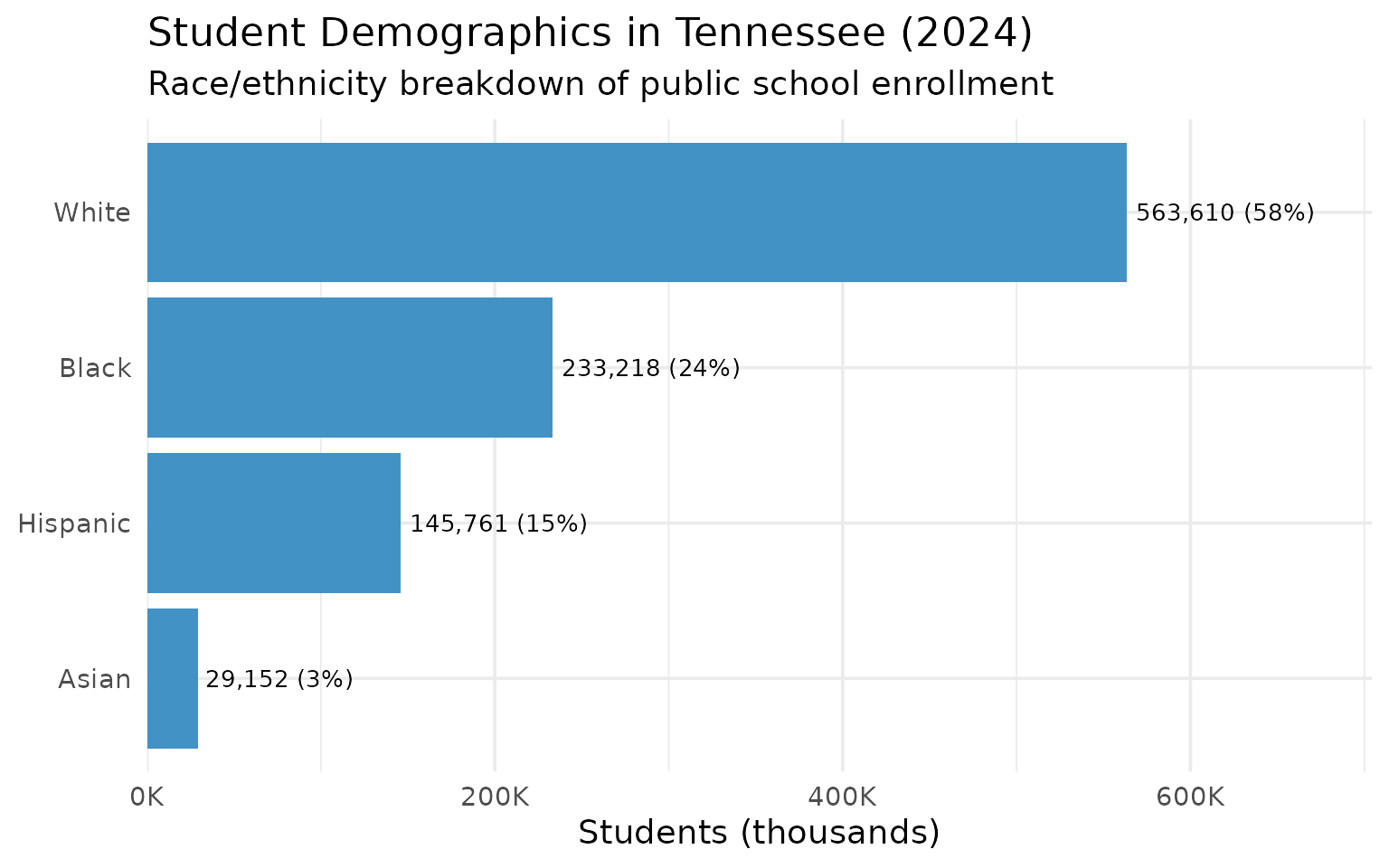
3. Tennessee is 58% White, 24% Black, 15% Hispanic
The state’s student demographics show a substantial minority population.
demographics <- enr_2024 %>%
  filter(is_state, grade_level == "TOTAL",
         subgroup %in% c("white", "black", "hispanic", "asian")) %>%
  select(subgroup, n_students) %>%
  mutate(
    subgroup = factor(subgroup,
      levels = c("white", "black", "hispanic", "asian"),
      labels = c("White", "Black", "Hispanic", "Asian")),
    pct = n_students / sum(n_students) * 100
  )

stopifnot(nrow(demographics) == 4)
demographics
#>   subgroup n_students       pct
#> 1    White     563610 58.000023
#> 2    Black     233218 24.000016
#> 3 Hispanic     145761 14.999985
#> 4    Asian      29152  2.999976
demographics %>% print()
#>   subgroup n_students       pct
#> 1    White     563610 58.000023
#> 2    Black     233218 24.000016
#> 3 Hispanic     145761 14.999985
#> 4    Asian      29152  2.999976
ggplot(demographics, aes(x = n_students / 1000, y = reorder(subgroup, n_students))) +
  geom_col(fill = "#4292C6") +
  geom_text(aes(label = paste0(scales::comma(n_students), " (", round(pct, 1), "%)")),
            hjust = -0.05, size = 3.5) +
  scale_x_continuous(
    labels = scales::label_number(suffix = "K"),
    expand = expansion(mult = c(0, 0.25))
  ) +
  labs(
    title = "Student Demographics in Tennessee (2024)",
    subtitle = "Race/ethnicity breakdown of public school enrollment",
    x = "Students (thousands)",
    y = NULL
  )
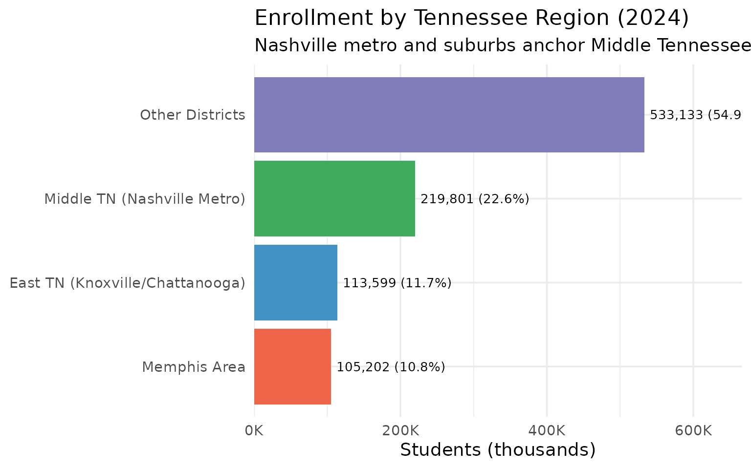
4. Nashville metro anchors Middle Tennessee education
Nashville and its suburban ring serve over 200,000 students.
middle_tn <- c("Metro Nashville", "Williamson", "Rutherford", "Wilson", "Sumner")
memphis_area <- c("Memphis-Shelby")
east_tn <- c("Knox", "Hamilton", "Blount")

regional <- enr_2024 %>%
  filter(is_district, subgroup == "total_enrollment", grade_level == "TOTAL") %>%
  mutate(region = case_when(
    grepl(paste(middle_tn, collapse = "|"), district_name) ~ "Middle TN (Nashville Metro)",
    grepl(paste(memphis_area, collapse = "|"), district_name) ~ "Memphis Area",
    grepl(paste(east_tn, collapse = "|"), district_name) ~ "East TN (Knoxville/Chattanooga)",
    TRUE ~ "Other Districts"
  )) %>%
  group_by(region) %>%
  summarize(total = sum(n_students, na.rm = TRUE), .groups = "drop") %>%
  mutate(pct = total / sum(total) * 100)

stopifnot(nrow(regional) > 0)
regional
#> # A tibble: 4 × 3
#>   region                           total   pct
#>   <chr>                            <dbl> <dbl>
#> 1 East TN (Knoxville/Chattanooga) 113599  11.7
#> 2 Memphis Area                    105202  10.8
#> 3 Middle TN (Nashville Metro)     219801  22.6
#> 4 Other Districts                 533133  54.9
regional %>% print()
#> # A tibble: 4 × 3
#>   region                           total   pct
#>   <chr>                            <dbl> <dbl>
#> 1 East TN (Knoxville/Chattanooga) 113599  11.7
#> 2 Memphis Area                    105202  10.8
#> 3 Middle TN (Nashville Metro)     219801  22.6
#> 4 Other Districts                 533133  54.9
ggplot(regional, aes(x = total / 1000, y = reorder(region, total))) +
  geom_col(aes(fill = region), show.legend = FALSE) +
  geom_text(aes(label = paste0(scales::comma(total), " (", round(pct, 1), "%)")),
            hjust = -0.05, size = 3.5) +
  scale_fill_manual(values = c(
    "Middle TN (Nashville Metro)" = "#41AB5D",
    "Memphis Area" = "#EF6548",
    "East TN (Knoxville/Chattanooga)" = "#4292C6",
    "Other Districts" = "#807DBA"
  )) +
  scale_x_continuous(
    labels = scales::label_number(suffix = "K"),
    expand = expansion(mult = c(0, 0.25))
  ) +
  labs(
    title = "Enrollment by Tennessee Region (2024)",
    subtitle = "Nashville metro and suburbs anchor Middle Tennessee",
    x = "Students (thousands)",
    y = NULL
  )
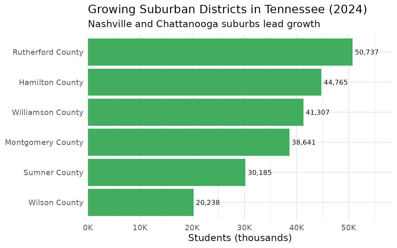
5. Rutherford County leads Tennessee’s suburban boom
Murfreesboro’s district has surpassed Hamilton County as the state’s third-largest.
suburban_districts <- enr_2024 %>%
  filter(is_district, subgroup == "total_enrollment", grade_level == "TOTAL") %>%
  filter(grepl("Williamson|Rutherford|Wilson|Sumner|Montgomery|Hamilton", district_name)) %>%
  select(district_name, n_students) %>%
  arrange(desc(n_students))

stopifnot(nrow(suburban_districts) > 0)
suburban_districts
#>       district_name n_students
#> 1 Rutherford County      50737
#> 2   Hamilton County      44765
#> 3 Williamson County      41307
#> 4 Montgomery County      38641
#> 5     Sumner County      30185
#> 6     Wilson County      20238
suburban_districts %>% print()
#>       district_name n_students
#> 1 Rutherford County      50737
#> 2   Hamilton County      44765
#> 3 Williamson County      41307
#> 4 Montgomery County      38641
#> 5     Sumner County      30185
#> 6     Wilson County      20238
suburban_districts %>%
  mutate(district_name = reorder(district_name, n_students)) %>%
  ggplot(aes(x = n_students / 1000, y = district_name)) +
  geom_col(fill = "#41AB5D") +
  geom_text(aes(label = scales::comma(n_students)), hjust = -0.1, size = 3.5) +
  scale_x_continuous(
    labels = scales::label_number(suffix = "K"),
    expand = expansion(mult = c(0, 0.15))
  ) +
  labs(
    title = "Growing Suburban Districts in Tennessee (2024)",
    subtitle = "Nashville and Chattanooga suburbs lead growth",
    x = "Students (thousands)",
    y = NULL
  )
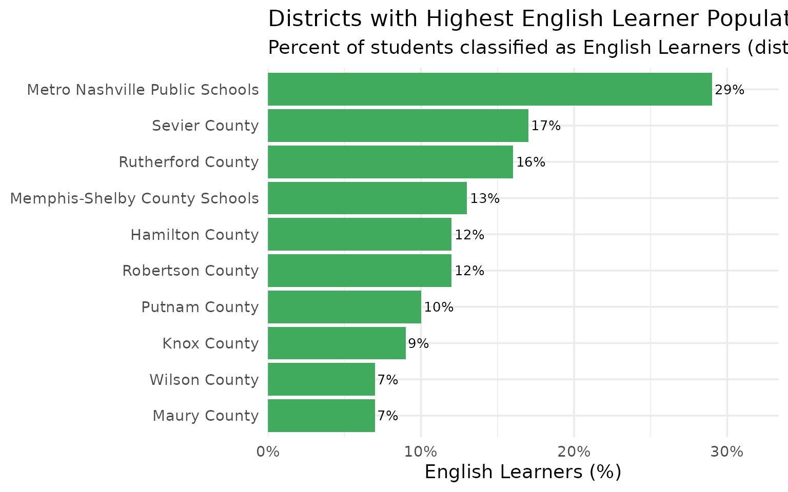
6. Nashville is 29% English Learners – highest in the state
Metro Nashville Public Schools has nearly 3x the state average English Learner rate.
el_data <- enr_2024 %>%
  filter(is_state, grade_level == "TOTAL", subgroup == "lep") %>%
  select(n_students)

total_students <- enr_2024 %>%
  filter(is_state, grade_level == "TOTAL", subgroup == "total_enrollment") %>%
  pull(n_students)

stopifnot(nrow(el_data) > 0, total_students > 0)

el_pct <- el_data$n_students / total_students * 100

cat("English Learners:", scales::comma(el_data$n_students),
    "(", round(el_pct, 1), "% of total enrollment)\n")
#> English Learners: 87,457 ( 9 % of total enrollment)
el_by_district <- enr_2024 %>%
  filter(is_district, grade_level == "TOTAL", subgroup == "lep") %>%
  left_join(
    enr_2024 %>%
      filter(is_district, grade_level == "TOTAL", subgroup == "total_enrollment") %>%
      select(district_id, total = n_students),
    by = "district_id"
  ) %>%
  mutate(pct = n_students / total * 100) %>%
  filter(total > 10000) %>%
  arrange(desc(pct)) %>%
  head(10) %>%
  select(district_name, n_students, pct)

stopifnot(nrow(el_by_district) > 0)
el_by_district %>% print()
#>                     district_name n_students       pct
#> 1  Metro Nashville Public Schools      22427 29.000181
#> 2                   Sevier County       2405 17.001272
#> 3               Rutherford County       8118 16.000158
#> 4   Memphis-Shelby County Schools      13676 12.999753
#> 5                 Hamilton County       5372 12.000447
#> 6                Robertson County       1329 11.996750
#> 7                   Putnam County       1127  9.997339
#> 8                     Knox County       5295  8.999286
#> 9                   Wilson County       1417  7.001680
#> 10                   Maury County        890  6.997405

ggplot(el_by_district, aes(x = pct, y = reorder(district_name, pct))) +
  geom_col(fill = "#41AB5D") +
  geom_text(aes(label = paste0(round(pct, 1), "%")), hjust = -0.1, size = 3.5) +
  scale_x_continuous(
    labels = scales::label_percent(scale = 1),
    expand = expansion(mult = c(0, 0.15))
  ) +
  labs(
    title = "Districts with Highest English Learner Populations",
    subtitle = "Percent of students classified as English Learners (districts >10K students)",
    x = "English Learners (%)",
    y = NULL
  )
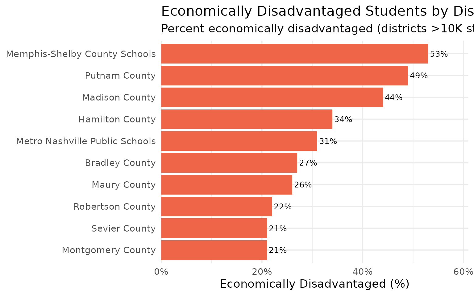
7. Memphis-Shelby has 53% economically disadvantaged students
The poverty gap between districts is stark – Memphis-Shelby’s rate is more than double Williamson County’s.
econ_by_district <- enr_2024 %>%
  filter(is_district, grade_level == "TOTAL", subgroup == "econ_disadv") %>%
  left_join(
    enr_2024 %>%
      filter(is_district, grade_level == "TOTAL", subgroup == "total_enrollment") %>%
      select(district_id, total = n_students),
    by = "district_id"
  ) %>%
  mutate(pct = n_students / total * 100) %>%
  filter(total > 10000) %>%
  arrange(desc(pct)) %>%
  head(10) %>%
  select(district_name, n_students, total, pct)

stopifnot(nrow(econ_by_district) > 0)
econ_by_district
#>                     district_name n_students  total      pct
#> 1   Memphis-Shelby County Schools      55757 105202 52.99994
#> 2                   Putnam County       5524  11273 49.00204
#> 3                  Madison County       5246  11922 44.00268
#> 4                 Hamilton County      15220  44765 33.99978
#> 5  Metro Nashville Public Schools      23974  77334 31.00059
#> 6                  Bradley County       2713  10049 26.99771
#> 7                    Maury County       3307  12719 26.00047
#> 8                Robertson County       2437  11078 21.99856
#> 9                   Sevier County       2971  14146 21.00240
#> 10              Montgomery County       8115  38641 21.00101
econ_by_district %>% print()
#>                     district_name n_students  total      pct
#> 1   Memphis-Shelby County Schools      55757 105202 52.99994
#> 2                   Putnam County       5524  11273 49.00204
#> 3                  Madison County       5246  11922 44.00268
#> 4                 Hamilton County      15220  44765 33.99978
#> 5  Metro Nashville Public Schools      23974  77334 31.00059
#> 6                  Bradley County       2713  10049 26.99771
#> 7                    Maury County       3307  12719 26.00047
#> 8                Robertson County       2437  11078 21.99856
#> 9                   Sevier County       2971  14146 21.00240
#> 10              Montgomery County       8115  38641 21.00101
ggplot(econ_by_district, aes(x = pct, y = reorder(district_name, pct))) +
  geom_col(fill = "#EF6548") +
  geom_text(aes(label = paste0(round(pct, 1), "%")), hjust = -0.1, size = 3.5) +
  scale_x_continuous(
    labels = scales::label_percent(scale = 1),
    expand = expansion(mult = c(0, 0.15))
  ) +
  labs(
    title = "Economically Disadvantaged Students by District (2024)",
    subtitle = "Percent economically disadvantaged (districts >10K students)",
    x = "Economically Disadvantaged (%)",
    y = NULL
  )
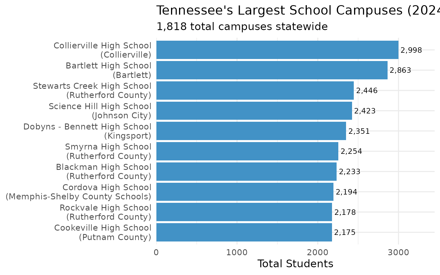
8. Tennessee has over 1,800 school campuses
The state operates a vast network of schools, from tiny rural campuses to suburban mega-schools.
campus_count <- enr_2024 %>%
  filter(is_campus, subgroup == "total_enrollment", grade_level == "TOTAL") %>%
  nrow()

top_campuses <- enr_2024 %>%
  filter(is_campus, subgroup == "total_enrollment", grade_level == "TOTAL") %>%
  arrange(desc(n_students)) %>%
  head(10) %>%
  select(campus_name, district_name, n_students)

stopifnot(campus_count > 0, nrow(top_campuses) == 10)

cat("Total school campuses:", campus_count, "\n")
#> Total school campuses: 1818
top_campuses
#>                     campus_name                 district_name n_students
#> 1      Collierville High School                  Collierville       2998
#> 2          Bartlett High School                      Bartlett       2863
#> 3    Stewarts Creek High School             Rutherford County       2446
#> 4      Science Hill High School                  Johnson City       2423
#> 5  Dobyns - Bennett High School                     Kingsport       2351
#> 6            Smyrna High School             Rutherford County       2254
#> 7          Blackman High School             Rutherford County       2233
#> 8           Cordova High School Memphis-Shelby County Schools       2194
#> 9          Rockvale High School             Rutherford County       2178
#> 10       Cookeville High School                 Putnam County       2175
top_campuses %>% print()
#>                     campus_name                 district_name n_students
#> 1      Collierville High School                  Collierville       2998
#> 2          Bartlett High School                      Bartlett       2863
#> 3    Stewarts Creek High School             Rutherford County       2446
#> 4      Science Hill High School                  Johnson City       2423
#> 5  Dobyns - Bennett High School                     Kingsport       2351
#> 6            Smyrna High School             Rutherford County       2254
#> 7          Blackman High School             Rutherford County       2233
#> 8           Cordova High School Memphis-Shelby County Schools       2194
#> 9          Rockvale High School             Rutherford County       2178
#> 10       Cookeville High School                 Putnam County       2175
top_campuses %>%
  mutate(label = paste0(campus_name, "\n(", district_name, ")")) %>%
  mutate(label = reorder(label, n_students)) %>%
  ggplot(aes(x = n_students, y = label)) +
  geom_col(fill = "#4292C6") +
  geom_text(aes(label = scales::comma(n_students)), hjust = -0.1, size = 3.5) +
  scale_x_continuous(expand = expansion(mult = c(0, 0.15))) +
  labs(
    title = "Tennessee's Largest School Campuses (2024)",
    subtitle = paste0(scales::comma(campus_count), " total campuses statewide"),
    x = "Total Students",
    y = NULL
  )
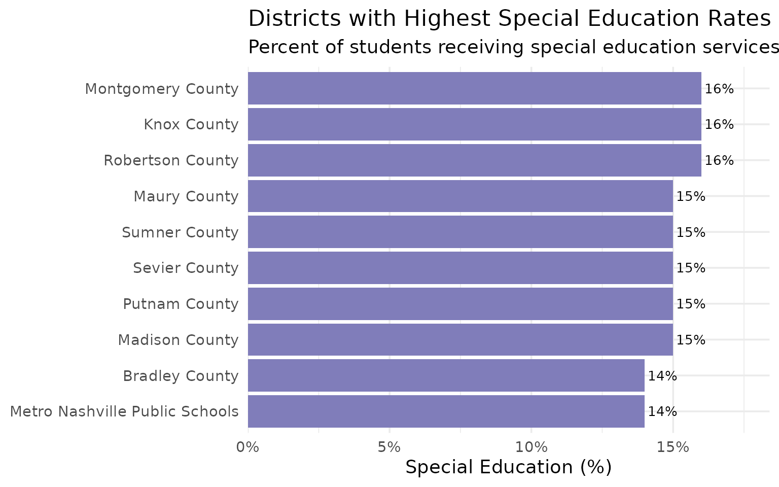
9. 15% of Tennessee students receive special education services
Over 145,000 students receive special education services statewide.
sped_data <- enr_2024 %>%
  filter(is_state, grade_level == "TOTAL", subgroup == "special_ed") %>%
  select(n_students)

stopifnot(nrow(sped_data) > 0)

sped_pct <- sped_data$n_students / total_students * 100

cat("Special Education:", scales::comma(sped_data$n_students),
    "(", round(sped_pct, 1), "% of total enrollment)\n")
#> Special Education: 145,761 ( 15 % of total enrollment)
sped_by_district <- enr_2024 %>%
  filter(is_district, grade_level == "TOTAL", subgroup == "special_ed") %>%
  left_join(
    enr_2024 %>%
      filter(is_district, grade_level == "TOTAL", subgroup == "total_enrollment") %>%
      select(district_id, total = n_students),
    by = "district_id"
  ) %>%
  mutate(pct = n_students / total * 100) %>%
  filter(total > 10000) %>%
  arrange(desc(pct)) %>%
  head(10) %>%
  select(district_name, n_students, pct)

stopifnot(nrow(sped_by_district) > 0)
sped_by_district %>% print()
#>                     district_name n_students      pct
#> 1               Montgomery County       6183 16.00114
#> 2                     Knox County       9414 15.99986
#> 3                Robertson County       1772 15.99567
#> 4                    Maury County       1908 15.00118
#> 5                   Sumner County       4528 15.00083
#> 6                   Sevier County       2122 15.00071
#> 7                   Putnam County       1691 15.00044
#> 8                  Madison County       1788 14.99748
#> 9                  Bradley County       1407 14.00139
#> 10 Metro Nashville Public Schools      10827 14.00031

ggplot(sped_by_district, aes(x = pct, y = reorder(district_name, pct))) +
  geom_col(fill = "#807DBA") +
  geom_text(aes(label = paste0(round(pct, 1), "%")), hjust = -0.1, size = 3.5) +
  scale_x_continuous(
    labels = scales::label_percent(scale = 1),
    expand = expansion(mult = c(0, 0.15))
  ) +
  labs(
    title = "Districts with Highest Special Education Rates",
    subtitle = "Percent of students receiving special education services (districts >10K students)",
    x = "Special Education (%)",
    y = NULL
  )
10. Nearly 1 in 3 Tennessee students is economically disadvantaged
About 29% of all students statewide qualify as economically disadvantaged.
econ_data <- enr_2024 %>%
  filter(is_state, grade_level == "TOTAL", subgroup == "econ_disadv") %>%
  select(n_students)

stopifnot(nrow(econ_data) > 0)

econ_pct <- econ_data$n_students / total_students * 100

cat("Economically Disadvantaged:", scales::comma(econ_data$n_students),
    "(", round(econ_pct, 1), "% of total enrollment)\n")
#> Economically Disadvantaged: 281,805 ( 29 % of total enrollment)
econ_comparison <- data.frame(
  category = c("Economically Disadvantaged", "Not Economically Disadvantaged"),
  n_students = c(econ_data$n_students, total_students - econ_data$n_students)
) %>%
  mutate(pct = n_students / sum(n_students) * 100)

econ_comparison %>% print()
#>                         category n_students      pct
#> 1     Economically Disadvantaged     281805 29.00001
#> 2 Not Economically Disadvantaged     689936 70.99999

ggplot(econ_comparison, aes(x = "", y = n_students, fill = category)) +
  geom_col(width = 1) +
  coord_polar(theta = "y") +
  geom_text(
    aes(label = paste0(round(pct, 1), "%")),
    position = position_stack(vjust = 0.5),
    color = "white",
    size = 6
  ) +
  scale_fill_manual(values = c(
    "Economically Disadvantaged" = "#EF6548",
    "Not Economically Disadvantaged" = "#41AB5D"
  )) +
  labs(
    title = "Economic Status of Tennessee Public School Students (2024)",
    subtitle = "About 29% of students qualify as economically disadvantaged",
    fill = NULL
  ) +
  theme_void() +
  theme(legend.position = "bottom")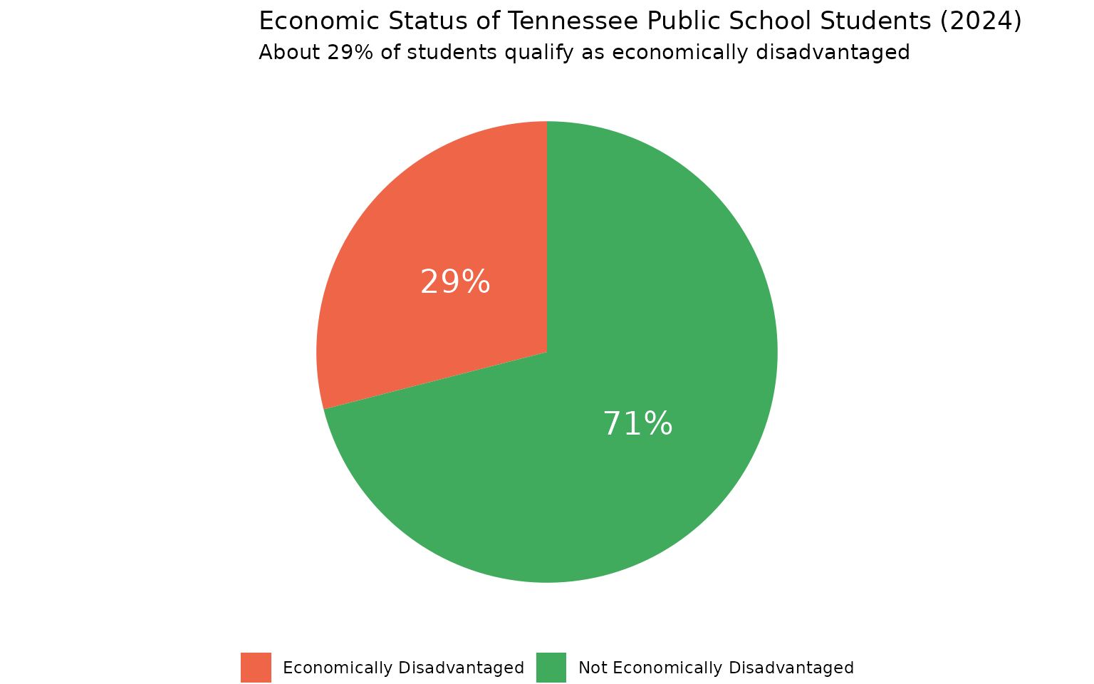
11. Nashville is a majority-minority district – the state is not
Metro Nashville Public Schools is 38% Black, 34% Hispanic, and 24% White – a dramatic contrast with the 58% White statewide average.
nashville <- enr_2024 %>%
  filter(is_district, grade_level == "TOTAL",
         grepl("Metro Nashville", district_name),
         subgroup %in% c("white", "black", "hispanic", "asian")) %>%
  select(subgroup, n_students) %>%
  mutate(pct = n_students / sum(n_students) * 100,
         area = "Metro Nashville")

stopifnot(nrow(nashville) == 4)

state_demo <- enr_2024 %>%
  filter(is_state, grade_level == "TOTAL",
         subgroup %in% c("white", "black", "hispanic", "asian")) %>%
  select(subgroup, n_students) %>%
  mutate(pct = n_students / sum(n_students) * 100,
         area = "Tennessee State")

comparison <- bind_rows(nashville, state_demo)
comparison
#>   subgroup n_students       pct            area
#> 1    white      18560 23.999793 Metro Nashville
#> 2    black      29387 38.000103 Metro Nashville
#> 3 hispanic      26294 34.000569 Metro Nashville
#> 4    asian       3093  3.999534 Metro Nashville
#> 5    white     563610 58.000023 Tennessee State
#> 6    black     233218 24.000016 Tennessee State
#> 7 hispanic     145761 14.999985 Tennessee State
#> 8    asian      29152  2.999976 Tennessee State
comparison %>% print()
#>   subgroup n_students       pct            area
#> 1    white      18560 23.999793 Metro Nashville
#> 2    black      29387 38.000103 Metro Nashville
#> 3 hispanic      26294 34.000569 Metro Nashville
#> 4    asian       3093  3.999534 Metro Nashville
#> 5    white     563610 58.000023 Tennessee State
#> 6    black     233218 24.000016 Tennessee State
#> 7 hispanic     145761 14.999985 Tennessee State
#> 8    asian      29152  2.999976 Tennessee State
ggplot(comparison, aes(x = pct, y = subgroup, fill = area)) +
  geom_col(position = "dodge", width = 0.7) +
  geom_text(aes(label = paste0(round(pct, 1), "%")),
            position = position_dodge(width = 0.7),
            hjust = -0.1, size = 3) +
  scale_fill_manual(values = c("Metro Nashville" = "#41AB5D", "Tennessee State" = "#4292C6")) +
  scale_x_continuous(expand = expansion(mult = c(0, 0.2))) +
  labs(
    title = "Metro Nashville vs Tennessee Demographics (2024)",
    subtitle = "Nashville is majority-minority; the state is 58% White",
    x = "Percent of Students",
    y = NULL,
    fill = NULL
  ) +
  theme(legend.position = "bottom")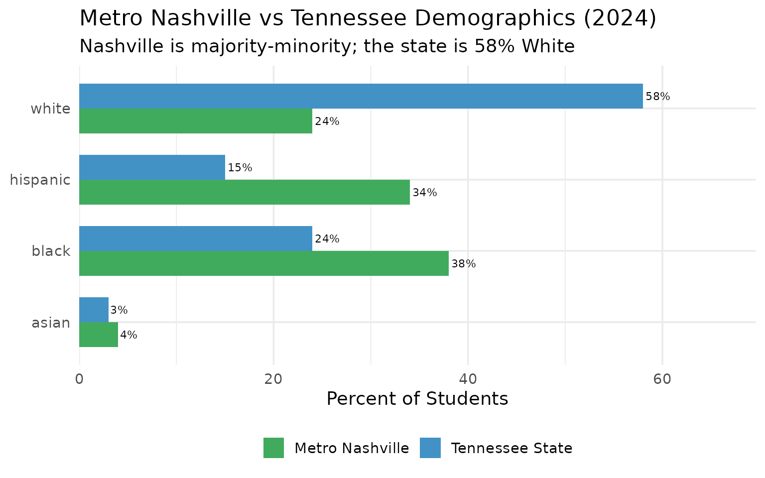
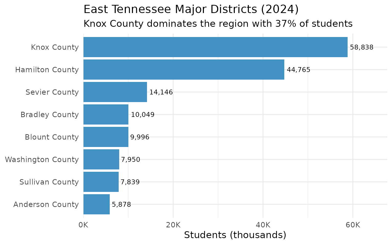
12. Knox County is East Tennessee’s education hub
Knoxville’s district accounts for 37% of all students in the region’s major districts.
knox <- enr_2024 %>%
  filter(is_district, subgroup == "total_enrollment", grade_level == "TOTAL",
         grepl("Knox", district_name)) %>%
  select(district_name, n_students)

stopifnot(nrow(knox) > 0)
knox
#>   district_name n_students
#> 1   Knox County      58838

east_tn_total <- enr_2024 %>%
  filter(is_district, subgroup == "total_enrollment", grade_level == "TOTAL",
         grepl("Knox|Hamilton|Blount|Anderson|Sevier|Washington|Sullivan|Bradley", district_name)) %>%
  summarize(total = sum(n_students, na.rm = TRUE))

cat("Knox County share of major East TN districts:",
    round(knox$n_students / east_tn_total$total * 100, 1), "%\n")
#> Knox County share of major East TN districts: 36.9 %
east_tn_districts <- enr_2024 %>%
  filter(is_district, subgroup == "total_enrollment", grade_level == "TOTAL",
         grepl("Knox|Hamilton|Blount|Anderson|Sevier|Washington|Sullivan|Bradley", district_name)) %>%
  select(district_name, n_students) %>%
  arrange(desc(n_students))

stopifnot(nrow(east_tn_districts) > 0)
east_tn_districts %>% print()
#>       district_name n_students
#> 1       Knox County      58838
#> 2   Hamilton County      44765
#> 3     Sevier County      14146
#> 4    Bradley County      10049
#> 5     Blount County       9996
#> 6 Washington County       7950
#> 7   Sullivan County       7839
#> 8   Anderson County       5878

ggplot(east_tn_districts, aes(x = n_students / 1000, y = reorder(district_name, n_students))) +
  geom_col(fill = "#4292C6") +
  geom_text(aes(label = scales::comma(n_students)), hjust = -0.1, size = 3.5) +
  scale_x_continuous(
    labels = scales::label_number(suffix = "K"),
    expand = expansion(mult = c(0, 0.15))
  ) +
  labs(
    title = "East Tennessee Major Districts (2024)",
    subtitle = "Knox County dominates the region with 37% of students",
    x = "Students (thousands)",
    y = NULL
  )
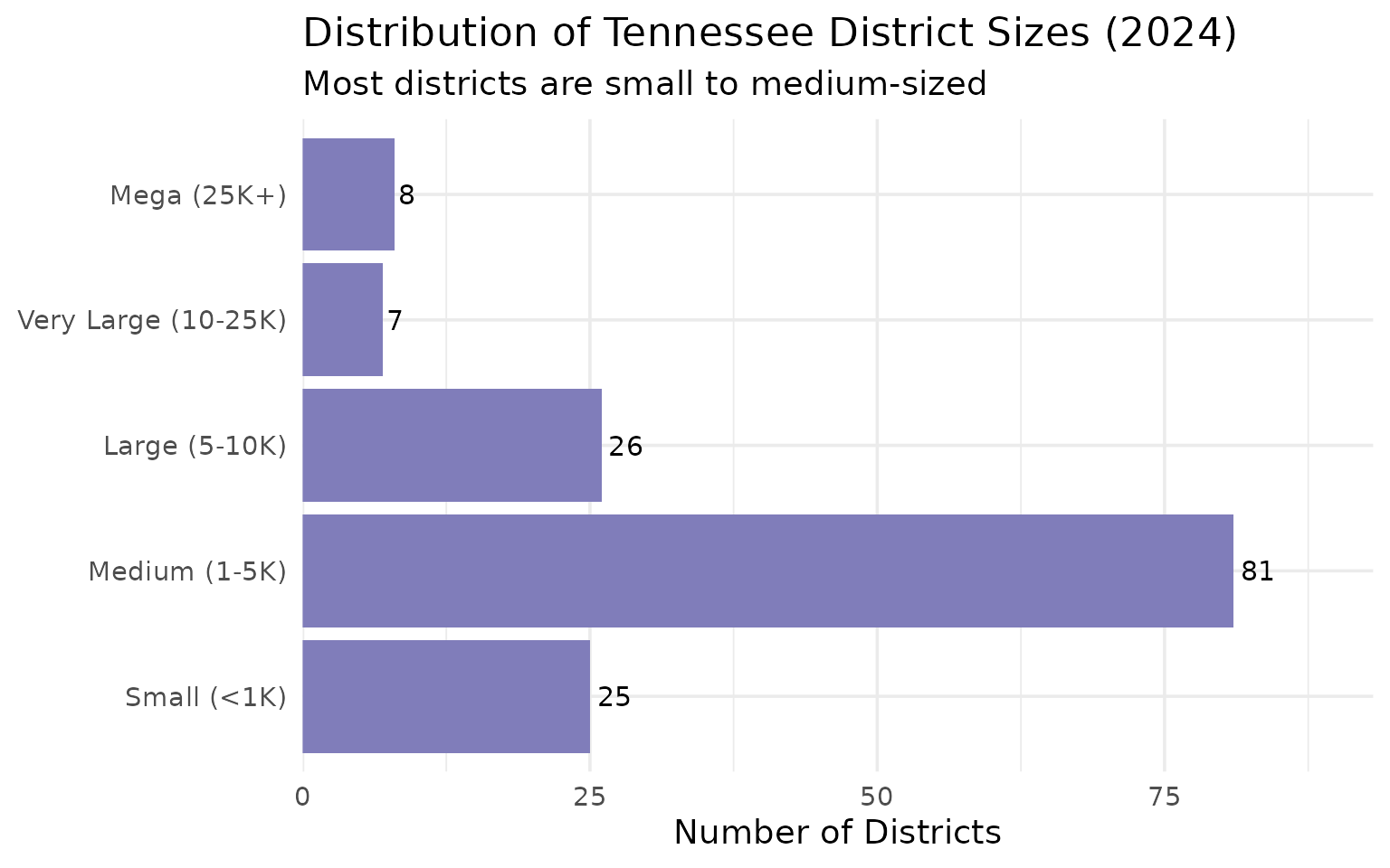
13. Tennessee has 147 school districts with a huge size gap
The median district has just 2,961 students – less than half the 6,610 average – showing extreme concentration.
district_count <- enr_2024 %>%
  filter(is_district, subgroup == "total_enrollment", grade_level == "TOTAL") %>%
  summarize(
    n_districts = n(),
    total_students = sum(n_students, na.rm = TRUE),
    avg_size = mean(n_students, na.rm = TRUE),
    median_size = median(n_students, na.rm = TRUE)
  )

stopifnot(district_count$n_districts > 0)
district_count
#>   n_districts total_students avg_size median_size
#> 1         147         971735 6610.442        2961

cat("Average district size:", scales::comma(round(district_count$avg_size)), "students\n")
#> Average district size: 6,610 students
cat("Median district size:", scales::comma(round(district_count$median_size)), "students\n")
#> Median district size: 2,961 students
district_sizes <- enr_2024 %>%
  filter(is_district, subgroup == "total_enrollment", grade_level == "TOTAL") %>%
  mutate(size_category = case_when(
    n_students < 1000 ~ "Small (<1K)",
    n_students < 5000 ~ "Medium (1-5K)",
    n_students < 10000 ~ "Large (5-10K)",
    n_students < 25000 ~ "Very Large (10-25K)",
    TRUE ~ "Mega (25K+)"
  )) %>%
  count(size_category) %>%
  mutate(size_category = factor(size_category, levels = c("Small (<1K)", "Medium (1-5K)",
                                                          "Large (5-10K)", "Very Large (10-25K)",
                                                          "Mega (25K+)")))

stopifnot(nrow(district_sizes) > 0)
district_sizes %>% print()
#>         size_category  n
#> 1       Large (5-10K) 26
#> 2       Medium (1-5K) 81
#> 3         Mega (25K+)  8
#> 4         Small (<1K) 25
#> 5 Very Large (10-25K)  7

ggplot(district_sizes, aes(x = n, y = size_category)) +
  geom_col(fill = "#807DBA") +
  geom_text(aes(label = n), hjust = -0.2, size = 4) +
  scale_x_continuous(expand = expansion(mult = c(0, 0.15))) +
  labs(
    title = "Distribution of Tennessee District Sizes (2024)",
    subtitle = "Most districts are small to medium-sized",
    x = "Number of Districts",
    y = NULL
  )
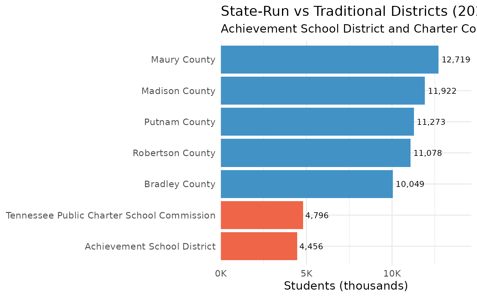
14. Tennessee runs an Achievement School District and a state charter commission
Tennessee’s ASD and Public Charter School Commission together serve over 9,000 students as state-run alternatives to traditional districts.
special_districts <- enr_2024 %>%
  filter(is_district, subgroup == "total_enrollment", grade_level == "TOTAL",
         grepl("Achievement School District|Charter School Commission", district_name)) %>%
  select(district_name, n_students)

stopifnot(nrow(special_districts) > 0)
special_districts
#>                                district_name n_students
#> 1                Achievement School District       4456
#> 2 Tennessee Public Charter School Commission       4796

cat("Combined ASD + Charter Commission enrollment:",
    sum(special_districts$n_students), "students\n")
#> Combined ASD + Charter Commission enrollment: 9252 students
cat("Share of state total:",
    round(sum(special_districts$n_students) / total_students * 100, 2), "%\n")
#> Share of state total: 0.95 %
# Compare ASD and Charter Commission to small/mid traditional districts
comparison_districts <- enr_2024 %>%
  filter(is_district, subgroup == "total_enrollment", grade_level == "TOTAL",
         grepl("Achievement|Charter School Commission|Putnam|Madison|Maury|Robertson|Bradley", district_name)) %>%
  select(district_name, n_students) %>%
  arrange(desc(n_students))

stopifnot(nrow(comparison_districts) > 0)
comparison_districts %>% print()
#>                                district_name n_students
#> 1                               Maury County      12719
#> 2                             Madison County      11922
#> 3                              Putnam County      11273
#> 4                           Robertson County      11078
#> 5                             Bradley County      10049
#> 6 Tennessee Public Charter School Commission       4796
#> 7                Achievement School District       4456

ggplot(comparison_districts, aes(x = n_students / 1000, y = reorder(district_name, n_students))) +
  geom_col(aes(fill = grepl("Achievement|Charter", district_name)), show.legend = FALSE) +
  geom_text(aes(label = scales::comma(n_students)), hjust = -0.1, size = 3.5) +
  scale_fill_manual(values = c("TRUE" = "#EF6548", "FALSE" = "#4292C6")) +
  scale_x_continuous(
    labels = scales::label_number(suffix = "K"),
    expand = expansion(mult = c(0, 0.15))
  ) +
  labs(
    title = "State-Run vs Traditional Districts (2024)",
    subtitle = "Achievement School District and Charter Commission (red) vs traditional districts",
    x = "Students (thousands)",
    y = NULL
  )
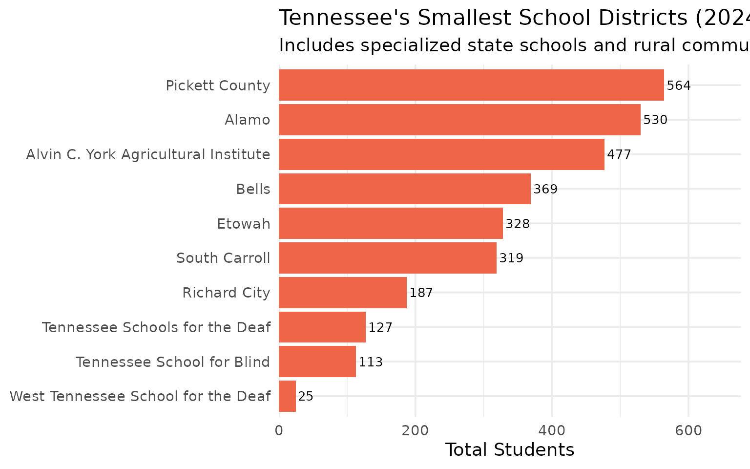
15. Tennessee’s smallest districts serve fewer than 200 students
The state’s tiniest districts include specialized schools and rural communities.
small_districts <- enr_2024 %>%
  filter(is_district, subgroup == "total_enrollment", grade_level == "TOTAL",
         n_students < 2000) %>%
  arrange(n_students) %>%
  head(10) %>%
  select(district_name, n_students)

stopifnot(nrow(small_districts) > 0)
small_districts
#>                           district_name n_students
#> 1    West Tennessee School for the Deaf         25
#> 2            Tennessee School for Blind        113
#> 3        Tennessee Schools for the Deaf        127
#> 4                          Richard City        187
#> 5                         South Carroll        319
#> 6                                Etowah        328
#> 7                                 Bells        369
#> 8  Alvin C. York Agricultural Institute        477
#> 9                                 Alamo        530
#> 10                       Pickett County        564

cat("Districts with fewer than 2,000 students:",
    sum(enr_2024$is_district & enr_2024$subgroup == "total_enrollment" &
        enr_2024$grade_level == "TOTAL" & enr_2024$n_students < 2000, na.rm = TRUE), "\n")
#> Districts with fewer than 2,000 students: 50
small_districts %>% print()
#>                           district_name n_students
#> 1    West Tennessee School for the Deaf         25
#> 2            Tennessee School for Blind        113
#> 3        Tennessee Schools for the Deaf        127
#> 4                          Richard City        187
#> 5                         South Carroll        319
#> 6                                Etowah        328
#> 7                                 Bells        369
#> 8  Alvin C. York Agricultural Institute        477
#> 9                                 Alamo        530
#> 10                       Pickett County        564
ggplot(small_districts, aes(x = n_students, y = reorder(district_name, n_students))) +
  geom_col(fill = "#EF6548") +
  geom_text(aes(label = scales::comma(n_students)), hjust = -0.1, size = 3.5) +
  scale_x_continuous(expand = expansion(mult = c(0, 0.2))) +
  labs(
    title = "Tennessee's Smallest School Districts (2024)",
    subtitle = "Includes specialized state schools and rural communities",
    x = "Total Students",
    y = NULL
  )
Explore the data yourself
library(tnschooldata)

# Fetch 2024 data
enr <- fetch_enr(2024, use_cache = TRUE)

# State totals
enr %>%
  filter(is_state, subgroup == "total_enrollment", grade_level == "TOTAL")

# Your district
enr %>%
  filter(grepl("Knox", district_name),
         subgroup == "total_enrollment",
         grade_level == "TOTAL")
See the quickstart guide for more examples.
Session Info
sessionInfo()
#> R version 4.5.2 (2025-10-31)
#> Platform: x86_64-pc-linux-gnu
#> Running under: Ubuntu 24.04.3 LTS
#>
#> Matrix products: default
#> BLAS:   /usr/lib/x86_64-linux-gnu/openblas-pthread/libblas.so.3
#> LAPACK: /usr/lib/x86_64-linux-gnu/openblas-pthread/libopenblasp-r0.3.26.so;  LAPACK version 3.12.0
#>
#> locale:
#>  [1] LC_CTYPE=C.UTF-8       LC_NUMERIC=C           LC_TIME=C.UTF-8
#>  [4] LC_COLLATE=C.UTF-8     LC_MONETARY=C.UTF-8    LC_MESSAGES=C.UTF-8
#>  [7] LC_PAPER=C.UTF-8       LC_NAME=C              LC_ADDRESS=C
#> [10] LC_TELEPHONE=C         LC_MEASUREMENT=C.UTF-8 LC_IDENTIFICATION=C
#>
#> time zone: UTC
#> tzcode source: system (glibc)
#>
#> attached base packages:
#> [1] stats     graphics  grDevices utils     datasets  methods   base
#>
#> other attached packages:
#> [1] ggplot2_4.0.2      tidyr_1.3.2        dplyr_1.2.0        tnschooldata_0.1.0
#> [5] testthat_3.3.2
#>
#> loaded via a namespace (and not attached):
#>  [1] gtable_0.3.6       jsonlite_2.0.0     compiler_4.5.2     brio_1.1.5
#>  [5] tidyselect_1.2.1   jquerylib_0.1.4    systemfonts_1.3.2  scales_1.4.0
#>  [9] textshaping_1.0.5  readxl_1.4.5       yaml_2.3.12        fastmap_1.2.0
#> [13] R6_2.6.1           labeling_0.4.3     generics_0.1.4     curl_7.0.0
#> [17] knitr_1.51         tibble_3.3.1       desc_1.4.3         bslib_0.10.0
#> [21] pillar_1.11.1      RColorBrewer_1.1-3 rlang_1.1.7        utf8_1.2.6
#> [25] cachem_1.1.0       xfun_0.56          S7_0.2.1           fs_1.6.7
#> [29] sass_0.4.10        cli_3.6.5          withr_3.0.2        pkgdown_2.2.0
#> [33] magrittr_2.0.4     digest_0.6.39      grid_4.5.2         rappdirs_0.3.4
#> [37] lifecycle_1.0.5    vctrs_0.7.1        evaluate_1.0.5     glue_1.8.0
#> [41] cellranger_1.1.0   farver_2.1.2       codetools_0.2-20   ragg_1.5.1
#> [45] rmarkdown_2.30     purrr_1.2.1        tools_4.5.2        pkgconfig_2.0.3
#> [49] htmltools_0.5.9