An R package for fetching and processing Texas school enrollment, graduation, and assessment data from the Texas Education Agency (TEA). Texas public schools enroll 5.5 million students across 1,200+ districts – the second-largest school system in the United States. One function call pulls it all into R.
This package is part of the njschooldata family of packages providing consistent access to state education data.
Documentation: https://almartin82.github.io/txschooldata/
Installation
R
# install.packages("remotes")
remotes::install_github("almartin82/txschooldata")What can you find with txschooldata?
library(txschooldata)
library(dplyr)
library(tidyr)
library(ggplot2)
library(scales)

# Fetch 5 years of enrollment data
enr <- fetch_enr_multi(2020:2024, use_cache = TRUE)
Here are fifteen narratives hiding in the numbers.
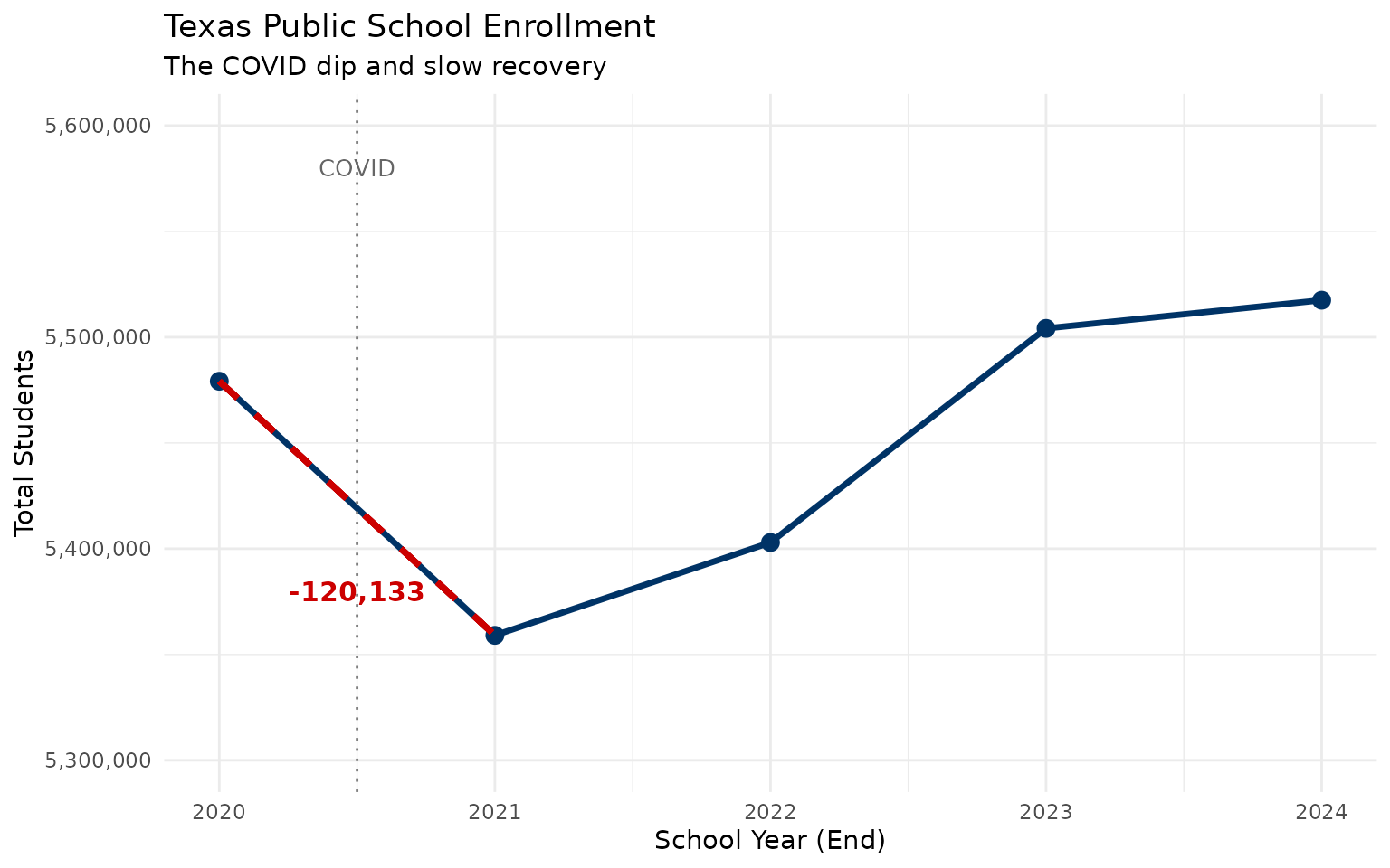
1. COVID erased a decade of growth in one year
state_trend <- enr %>%
  filter(is_state, subgroup == "total_enrollment", grade_level == "TOTAL") %>%
  select(end_year, n_students) %>%
  arrange(end_year) %>%
  mutate(
    change = n_students - lag(n_students),
    pct_change = round(change / lag(n_students) * 100, 2)
  )

stopifnot(nrow(state_trend) > 0)
print(state_trend)
#>   end_year n_students  change pct_change
#> 1     2020    5479173      NA         NA
#> 2     2021    5359040 -120133      -2.19
#> 3     2022    5402928   43888       0.82
#> 4     2023    5504150  101222       1.87
#> 5     2024    5517464   13314       0.24
-120,133 students vanished between 2020 and 2021 – equivalent to the entire enrollment of El Paso ISD.
2. One in four students is now an English learner
lep_trend <- enr %>%
  filter(is_state, subgroup == "lep", grade_level == "TOTAL") %>%
  select(end_year, n_students, pct) %>%
  mutate(pct_display = round(pct * 100, 1))

stopifnot(nrow(lep_trend) > 0)
print(lep_trend %>% select(end_year, n_students, pct_display))
#>   end_year n_students pct_display
#> 1     2020    1112674        20.3
#> 2     2021    1108207        20.7
#> 3     2022    1171661        21.7
#> 4     2023    1269408        23.1
#> 5     2024    1344804        24.4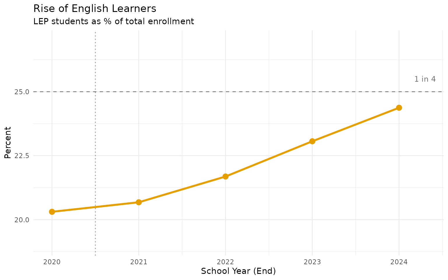
From 20.3% to 24.4% in five years. Schools need more ESL teachers than ever.
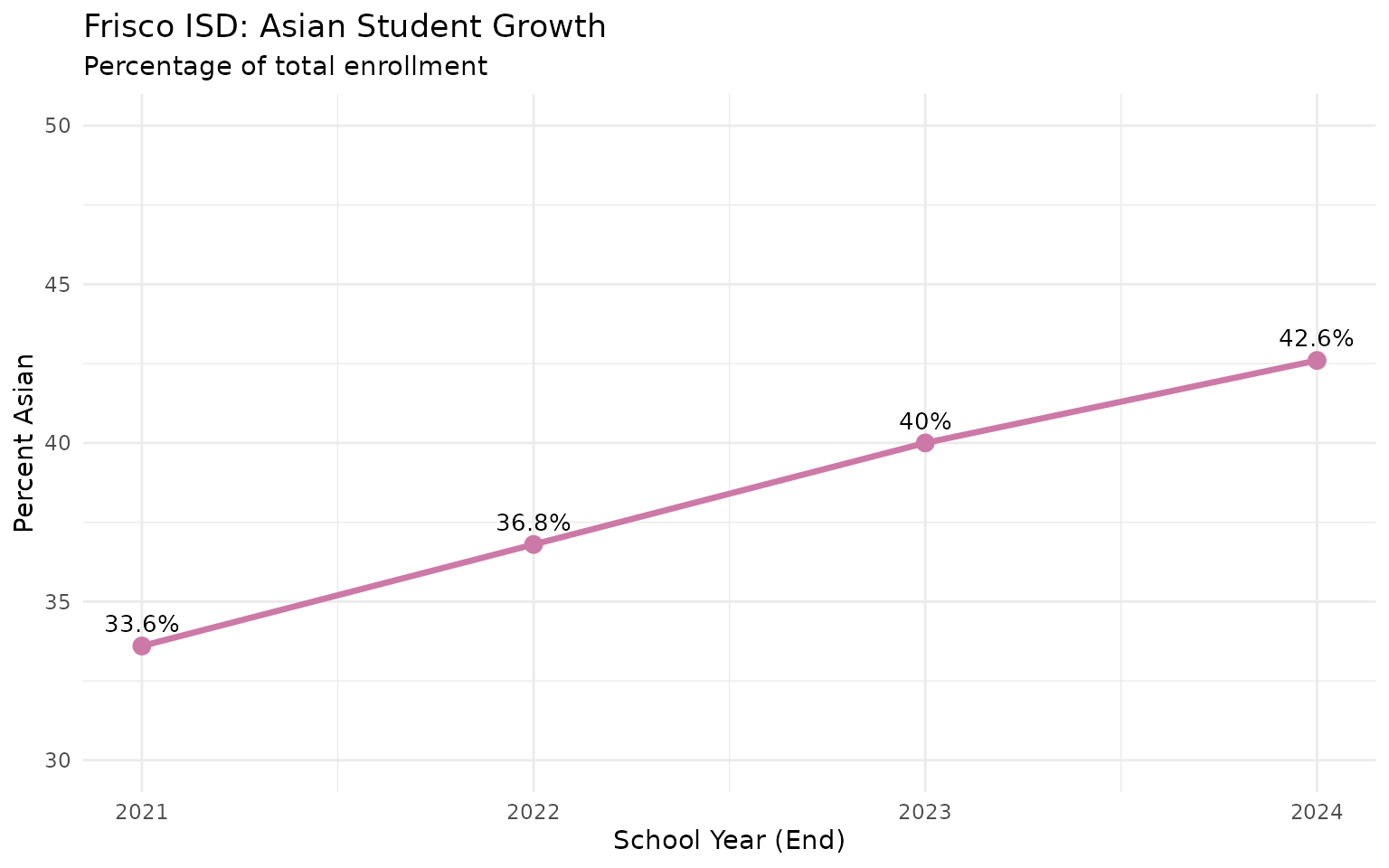
3. Coppell ISD is Texas’s first Asian-majority district
# Districts with highest Asian percentage
asian_top <- enr %>%
  filter(is_district, subgroup == "asian", grade_level == "TOTAL", end_year == 2024) %>%
  inner_join(
    enr %>% filter(is_district, subgroup == "total_enrollment",
                   grade_level == "TOTAL", end_year == 2024) %>%
      select(district_id, total = n_students),
    by = "district_id"
  ) %>%
  filter(total >= 10000) %>%
  arrange(desc(pct)) %>%
  select(district_name, total, n_students, pct) %>%
  mutate(pct = round(pct * 100, 1)) %>%
  head(10)

stopifnot(nrow(asian_top) > 0)
print(asian_top)
#>     district_name total n_students  pct
#> 1     COPPELL ISD 13394       7591 56.7
#> 2      FRISCO ISD 66551      28349 42.6
#> 3     PROSPER ISD 28394       8312 29.3
#> 4       ALLEN ISD 21319       6201 29.1
#> 5   FORT BEND ISD 80034      22080 27.6
#> 6       PLANO ISD 47753      11207 23.5
#> 7  ROUND ROCK ISD 46042      10126 22.0
#> 8        KATY ISD 94589      16311 17.2
#> 9       WYLIE ISD 19166       3227 16.8
#> 10 LEWISVILLE ISD 48356       8123 16.8
56.7% Asian. Frisco ISD jumped from 33.6% to 42.6% in just three years.
4. Fort Worth ISD lost 14% of its students
# Calculate 2020-2024 changes using district_id (2020 data has NA names)
d2020 <- enr %>%
  filter(is_district, subgroup == "total_enrollment",
         grade_level == "TOTAL", end_year == 2020) %>%
  select(district_id, n_2020 = n_students)

d2024 <- enr %>%
  filter(is_district, subgroup == "total_enrollment",
         grade_level == "TOTAL", end_year == 2024) %>%
  select(district_id, district_name, n_2024 = n_students)

losses <- d2020 %>%
  inner_join(d2024, by = "district_id") %>%
  mutate(
    change = n_2024 - n_2020,
    pct_change = round((change / n_2020) * 100, 1)
  )

# Largest percentage losses among big districts
top_losses <- losses %>%
  filter(n_2020 >= 10000) %>%
  arrange(pct_change) %>%
  select(district_name, n_2020, n_2024, change, pct_change) %>%
  head(10)

stopifnot(nrow(top_losses) > 0)
print(top_losses)
#>      district_name n_2020 n_2024 change pct_change
#> 1   FORT WORTH ISD  82704  70903 -11801      -14.3
#> 2       ALDINE ISD  67130  57737  -9393      -14.0
#> 3  BROWNSVILLE ISD  42989  37032  -5957      -13.9
#> 4   HARLANDALE ISD  13654  11781  -1873      -13.7
#> 5       YSLETA ISD  40404  34875  -5529      -13.7
#> 6       LAREDO ISD  23665  20557  -3108      -13.1
#> 7        ALIEF ISD  45281  39451  -5830      -12.9
#> 8      HOUSTON ISD 209309 183603 -25706      -12.3
#> 9      LA JOYA ISD  27276  23995  -3281      -12.0
#> 10     ABILENE ISD  16456  14482  -1974      -12.0
Urban districts are bleeding students to suburbs and charters.
5. IDEA Public Schools grew 55% in five years
# Use district_id join to include 2020 (which has NA district_name)
idea_trend <- losses %>%
  filter(grepl("IDEA", district_name))

stopifnot(nrow(idea_trend) > 0)
print(idea_trend %>% select(district_name, n_2020, n_2024, change, pct_change))
#>         district_name n_2020 n_2024 change pct_change
#> 1 IDEA PUBLIC SCHOOLS  49480  76819  27339       55.3

# Year-by-year for 2021-2024 (name filter works for these years)
idea_yearly <- enr %>%
  filter(district_name == "IDEA PUBLIC SCHOOLS", is_district,
         subgroup == "total_enrollment", grade_level == "TOTAL") %>%
  select(end_year, n_students) %>%
  arrange(end_year)

stopifnot(nrow(idea_yearly) > 0)
print(idea_yearly)
#>   end_year n_students
#> 1     2021      62158
#> 2     2022      67988
#> 3     2023      74217
#> 4     2024      76819
From 49,480 to 76,819 students (+55.3%). Charter networks are reshaping Texas education.
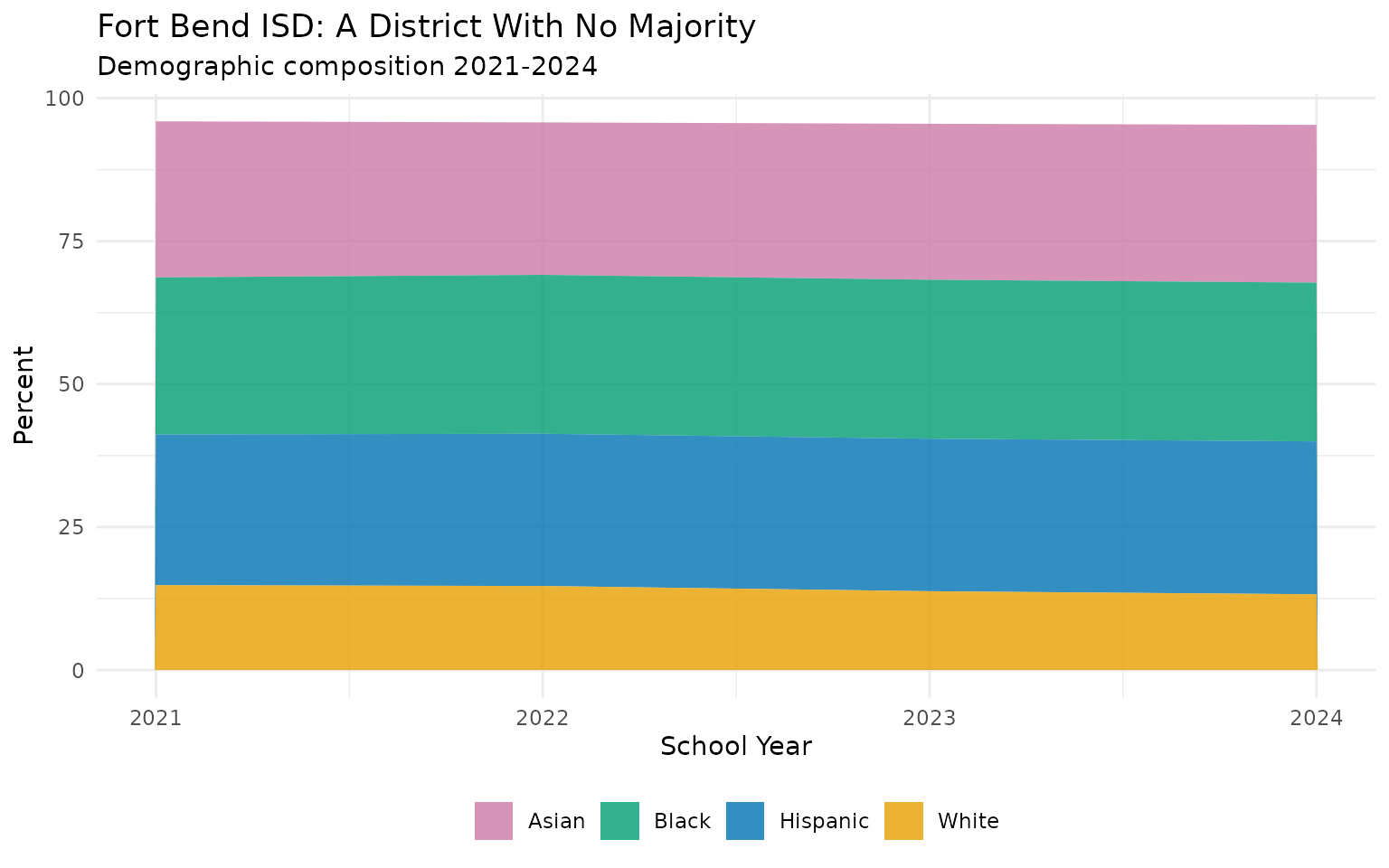
6. Fort Bend ISD has no racial majority
fb_demo <- enr %>%
  filter(district_name == "FORT BEND ISD", is_district, grade_level == "TOTAL",
         subgroup %in% c("white", "black", "hispanic", "asian")) %>%
  select(end_year, subgroup, pct) %>%
  mutate(pct = round(pct * 100, 1)) %>%
  pivot_wider(names_from = subgroup, values_from = pct)

stopifnot(nrow(fb_demo) > 0)
print(fb_demo)
#> # A tibble: 4 × 5
#>   end_year white black hispanic asian
#>      <int> <dbl> <dbl>    <dbl> <dbl>
#> 1     2021  14.8  27.5     26.4  27.3
#> 2     2022  14.7  27.8     26.6  26.7
#> 3     2023  13.8  27.8     26.7  27.3
#> 4     2024  13.2  27.8     26.7  27.6
No group exceeds 28%. One of the most diverse large districts in America.
7. Kindergarten enrollment dropped 5.8%
grade_trend <- enr %>%
  filter(is_state, subgroup == "total_enrollment",
         grade_level %in% c("PK", "K", "01", "05", "09", "12")) %>%
  select(end_year, grade_level, n_students) %>%
  pivot_wider(names_from = end_year, values_from = n_students) %>%
  mutate(
    change = `2024` - `2020`,
    pct_change = round(change / `2020` * 100, 1)
  )

stopifnot(nrow(grade_trend) > 0)
print(grade_trend)
#> # A tibble: 6 × 8
#>   grade_level `2020` `2021` `2022` `2023` `2024` change pct_change
#>   <chr>        <dbl>  <dbl>  <dbl>  <dbl>  <dbl>  <dbl>      <dbl>
#> 1 PK          248413 196560 222767 243493 247979   -434       -0.2
#> 2 K           383585 360865 370054 367180 361329 -22256       -5.8
#> 3 01          391175 380973 384494 399048 385096  -6079       -1.6
#> 4 05          417272 395436 387945 395111 399200 -18072       -4.3
#> 5 09          448929 436396 475437 477875 472595  23666        5.3
#> 6 12          352258 362888 360056 364317 365788  13530        3.8
-22,256 kindergartners since 2020. The pipeline is narrowing.
8. 62% of students are economically disadvantaged
econ_trend <- enr %>%
  filter(is_state, subgroup == "econ_disadv", grade_level == "TOTAL") %>%
  select(end_year, n_students, pct) %>%
  mutate(pct = round(pct * 100, 1))

stopifnot(nrow(econ_trend) > 0)
print(econ_trend)
#>   end_year n_students  pct
#> 1     2020    3303974 60.3
#> 2     2021    3229178 60.3
#> 3     2022    3278452 60.7
#> 4     2023    3415987 62.1
#> 5     2024    3434955 62.3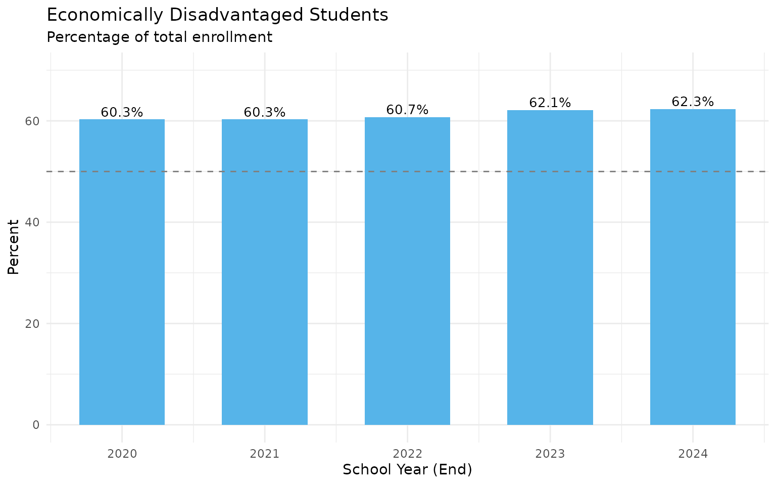
Up from 60.3%. Nearly two-thirds of Texas students qualify.
9. White students dropped below 25%
demo_shift <- enr %>%
  filter(is_state, grade_level == "TOTAL",
         subgroup %in% c("white", "black", "hispanic", "asian", "multiracial")) %>%
  select(end_year, subgroup, pct) %>%
  mutate(pct = round(pct * 100, 1)) %>%
  pivot_wider(names_from = subgroup, values_from = pct)

stopifnot(nrow(demo_shift) > 0)
print(demo_shift)
#> # A tibble: 5 × 6
#>   end_year white black hispanic asian multiracial
#>      <int> <dbl> <dbl>    <dbl> <dbl>       <dbl>
#> 1     2020  27    12.6     52.8   4.6         2.5
#> 2     2021  26.5  12.7     52.9   4.7         2.7
#> 3     2022  26.3  12.8     52.8   4.8         2.9
#> 4     2023  25.6  12.8     53     5.1         3
#> 5     2024  25    12.8     53.2   5.4         3.1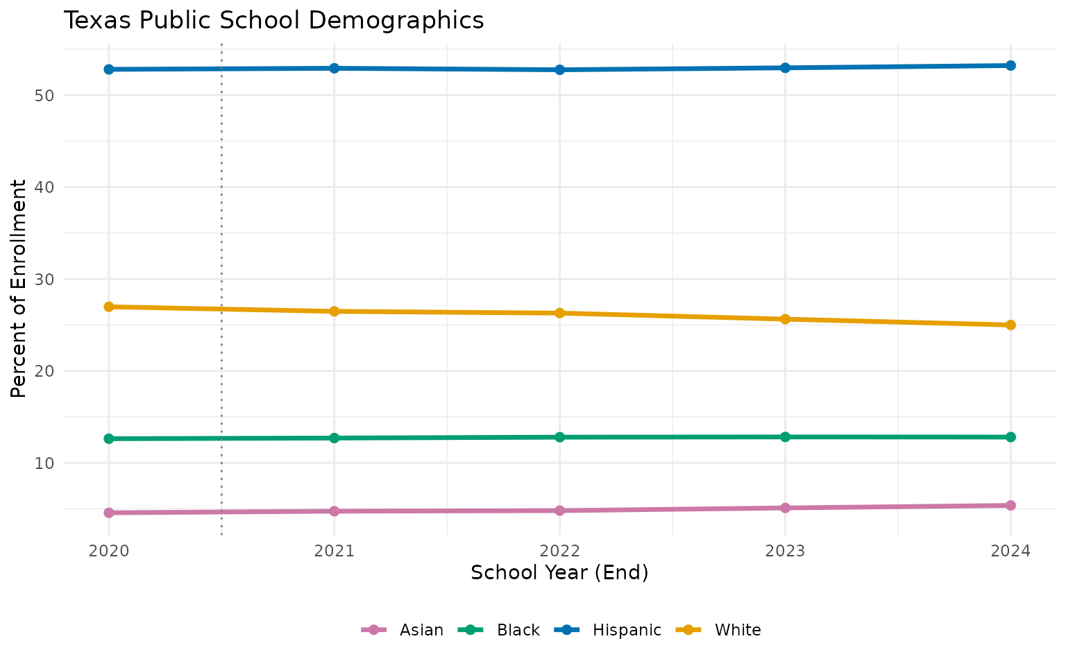
Hispanic students are now 53.2% of enrollment.
10. 439 districts now have Hispanic majorities
hisp_majority <- enr %>%
  filter(is_district, subgroup == "hispanic", grade_level == "TOTAL") %>%
  mutate(majority = pct > 0.5) %>%
  group_by(end_year) %>%
  summarize(
    total_districts = n(),
    hispanic_majority = sum(majority),
    pct_majority = round(hispanic_majority / total_districts * 100, 1),
    .groups = "drop"
  )

stopifnot(nrow(hisp_majority) > 0)
print(hisp_majority)
#> # A tibble: 5 × 4
#>   end_year total_districts hispanic_majority pct_majority
#>      <int>           <int>             <int>        <dbl>
#> 1     2020            1202               419         34.9
#> 2     2021            1204               428         35.5
#> 3     2022            1207               433         35.9
#> 4     2023            1209               438         36.2
#> 5     2024            1207               439         36.4
Up from 419 in 2020. Now 36.4% of all Texas school districts.
11. Houston ISD vs Dallas ISD: two giants, two trajectories
# Use district_id to include 2020 (which has NA district_name)
big_two_ids <- c("101912", "057905")  # Houston ISD, Dallas ISD

big_two <- enr %>%
  filter(is_district, subgroup == "total_enrollment", grade_level == "TOTAL",
         district_id %in% big_two_ids) %>%
  mutate(district_label = case_when(
    district_id == "101912" ~ "HOUSTON ISD",
    district_id == "057905" ~ "DALLAS ISD"
  )) %>%
  select(end_year, district_label, n_students) %>%
  pivot_wider(names_from = district_label, values_from = n_students) %>%
  arrange(end_year) %>%
  mutate(
    houston_change = `HOUSTON ISD` - lag(`HOUSTON ISD`),
    dallas_change = `DALLAS ISD` - lag(`DALLAS ISD`)
  )

stopifnot(nrow(big_two) > 0)
print(big_two)
#> # A tibble: 5 × 5
#>   end_year `DALLAS ISD` `HOUSTON ISD` houston_change dallas_change
#>      <int>        <dbl>         <dbl>          <dbl>         <dbl>
#> 1     2020       153784        209309             NA            NA
#> 2     2021       145105        196550         -12759         -8679
#> 3     2022       143430        193727          -2823         -1675
#> 4     2023       141042        189290          -4437         -2388
#> 5     2024       139096        183603          -5687         -1946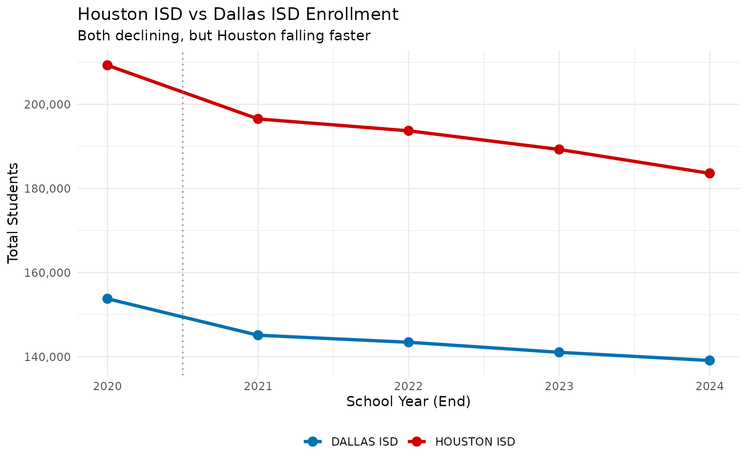
Houston lost 25,706 students (-12.3%) vs Dallas’s 14,688 (-9.5%) between 2020 and 2024.
12. Nearly 1 in 7 students receives special education
sped_2024 <- enr %>%
  filter(is_state, subgroup == "special_ed", grade_level == "TOTAL", end_year == 2024) %>%
  select(end_year, n_students, pct) %>%
  mutate(pct_display = round(pct * 100, 1))

stopifnot(nrow(sped_2024) > 0)
print(sped_2024 %>% select(end_year, n_students, pct_display))
#>   end_year n_students pct_display
#> 1     2024     764858        13.9
764,858 students (13.9%) receive special education services in 2024.
13. Suburban boomtowns are reshaping Texas education
# Top growing large districts (using district_id join for accurate 2020-2024 comparison)
suburban_growth <- losses %>%
  filter(n_2020 >= 5000) %>%
  arrange(desc(pct_change)) %>%
  select(district_name, n_2020, n_2024, change, pct_change) %>%
  head(10)

stopifnot(nrow(suburban_growth) > 0)
print(suburban_growth)
#>                  district_name n_2020 n_2024 change pct_change
#> 1               HALLSVILLE ISD  11452  21266   9814       85.7
#> 2                  PROSPER ISD  16789  28394  11605       69.1
#> 3                PRINCETON ISD   5414   8671   3257       60.2
#> 4                CLEVELAND ISD   7559  11945   4386       58.0
#> 5          IDEA PUBLIC SCHOOLS  49480  76819  27339       55.3
#> 6            MEDINA VALLEY ISD   5847   8656   2809       48.0
#> 7         PREMIER HIGH SCHOOLS   5345   7819   2474       46.3
#> 8  YES PREP PUBLIC SCHOOLS INC  12074  17622   5548       45.9
#> 9                   FORNEY ISD  11944  16962   5018       42.0
#> 10              ROYSE CITY ISD   6585   9338   2753       41.8
Hallsville ISD nearly doubled (+85.7%), Prosper ISD grew 69.1%. While urban cores lose students, suburban boomtowns absorb the growth.
14. Pre-K enrollment still hasn’t recovered from COVID
pk_trend <- enr %>%
  filter(is_state, subgroup == "total_enrollment", grade_level == "PK") %>%
  select(end_year, n_students) %>%
  arrange(end_year) %>%
  mutate(
    change = n_students - lag(n_students),
    pct_change = round(change / lag(n_students) * 100, 1),
    vs_2020 = n_students - first(n_students)
  )

stopifnot(nrow(pk_trend) > 0)
print(pk_trend)
#>   end_year n_students change pct_change vs_2020
#> 1     2020     248413     NA         NA       0
#> 2     2021     196560 -51853      -20.9  -51853
#> 3     2022     222767  26207       13.3  -25646
#> 4     2023     243493  20726        9.3   -4920
#> 5     2024     247979   4486        1.8    -434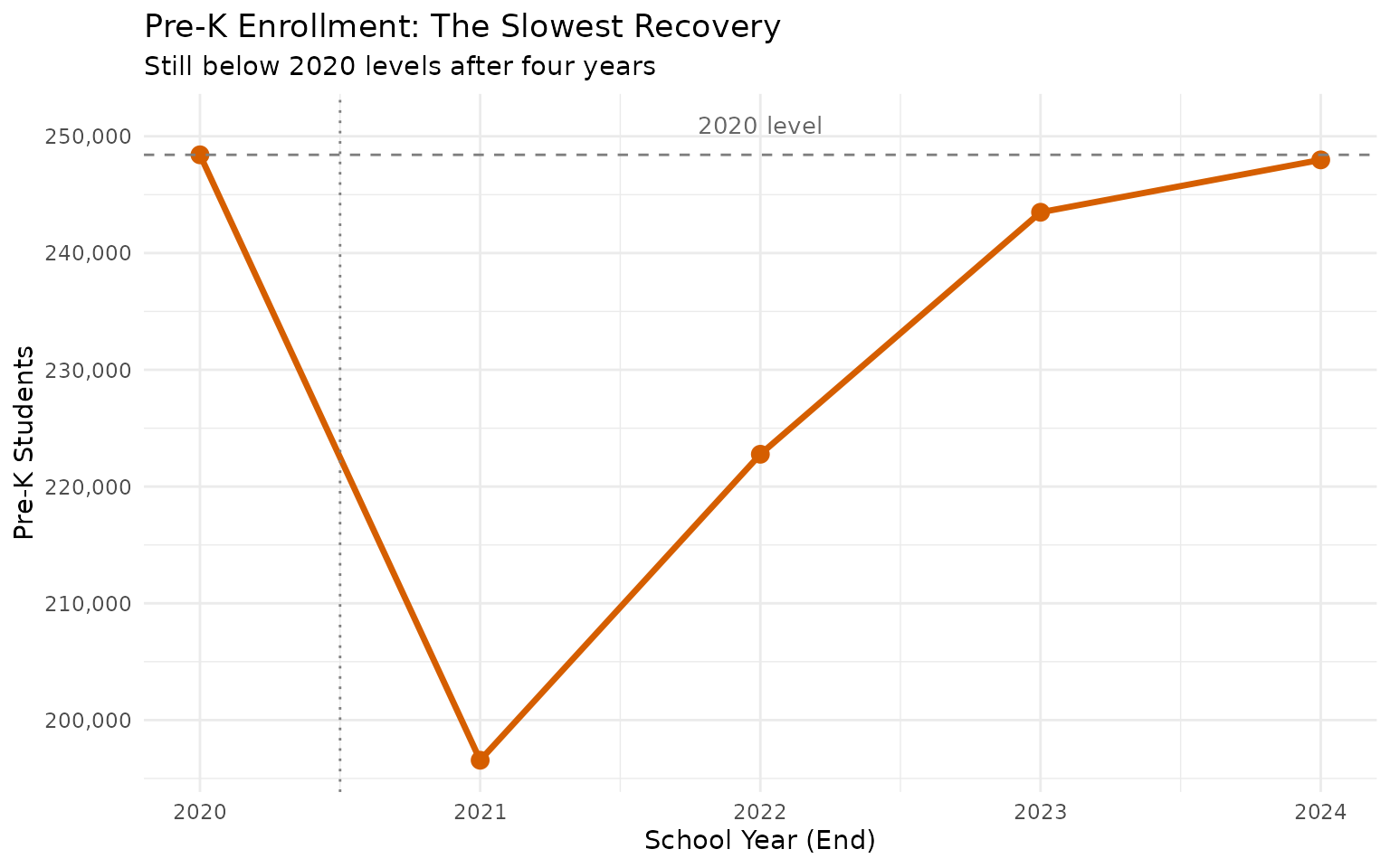
Pre-K cratered 21% during COVID. By 2024 it has clawed back to 247,979 – still 434 students short of 2020 levels.
15. Multiracial students are the fastest-growing demographic
multi_trend <- enr %>%
  filter(is_state, subgroup == "multiracial", grade_level == "TOTAL") %>%
  select(end_year, n_students, pct) %>%
  mutate(pct_display = round(pct * 100, 1))

stopifnot(nrow(multi_trend) > 0)
print(multi_trend %>% select(end_year, n_students, pct_display))
#>   end_year n_students pct_display
#> 1     2020     138434         2.5
#> 2     2021     143368         2.7
#> 3     2022     155887         2.9
#> 4     2023     166128         3.0
#> 5     2024     173425         3.1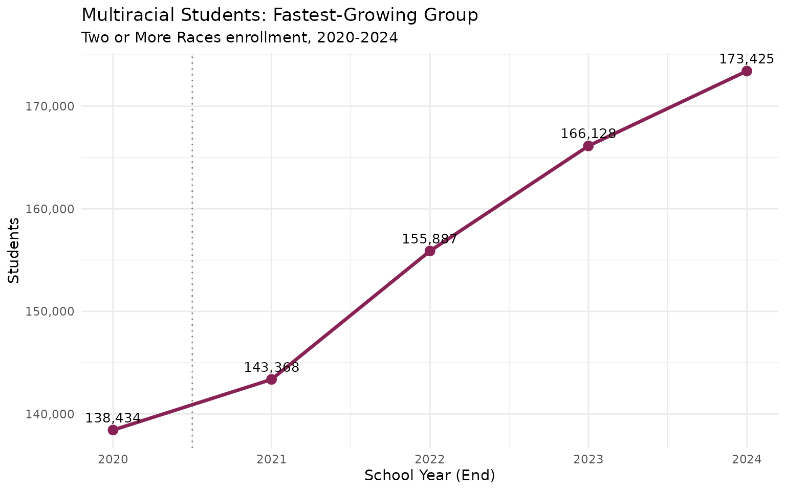
From 138,434 to 173,425 – a 25% increase in raw numbers. The fastest-growing demographic group in Texas.
Graduation rates
Track four-year longitudinal graduation rates for the Class of 2003-2024:
library(txschooldata)

# Get Class of 2024 graduation rates
grad <- fetch_grad(2024, use_cache = TRUE)

# State graduation rate by subgroup
grad |>
  filter(type == "State") |>
  select(subgroup, grad_rate) |>
  arrange(desc(grad_rate))
#>           subgroup grad_rate
#> 1            asian  95.59655
#> 2           female  95.40719
#> 3            white  94.74369
#> 4     all_students  94.39027
#> 5         hispanic  93.69867
#> 6             male  93.38859
#> 7      econ_disadv  93.24518
#> 8      multiracial  93.09000
#> 9          at_risk  92.12205
#> 10             lep  91.25872
#> 11      special_ed  87.80512
#> 12           black        NA
#> 13 native_american        NA
Data available for all students plus race/ethnicity, gender, and special populations (economically disadvantaged, special education, LEP, at-risk).
Data availability
This package pulls from three TEA reporting systems:
| System | Years | Notes |
|---|---|---|
| AEIS CGI | 1997-2002 | Older AEIS format via CGI endpoint |
| AEIS SAS | 2003-2012 | Academic Excellence Indicator System |
| TAPR | 2013-2025 | Texas Academic Performance Reports |
All data is fetched directly from TEA servers – no manual downloads required.
What’s included
Enrollment data: - Levels: State, district (~1,200), and campus (~9,000) - Demographics: White, Black, Hispanic, Asian, American Indian, Pacific Islander, Two or More Races - Special populations: Economically disadvantaged, LEP/English learners, Special education, At-risk, Gifted - Grade levels: Early Education (EE) through Grade 12, plus totals
Graduation rate data: - Years: Class of 2003-2024 (four-year longitudinal rates) - Levels: State, district, campus - Subgroups: All students, race/ethnicity, gender, special populations - Note: Uses federal calculation for consistency across years
Data notes
-
IDs: District IDs are 6 digits (e.g.,
101912for Houston ISD). Campus IDs are 9 digits (district + 3-digit campus number). -
Tidy format: By default,
fetch_enr()returns long/tidy data withsubgroup,grade_level, andn_studentscolumns. Usetidy = FALSEfor wide format. -
Percentages: The
pctcolumn is a proportion (0-1), not a percentage. Multiply by 100 for display. -
Caching: Data is cached locally after first download. Use
use_cache = FALSEto force refresh. - Suppression: TEA applies data masking to protect student privacy for small subgroups.
Caveats
- Asian/Pacific Islander: Pre-2011 data combines Asian and Pacific Islander into a single “asian” category. Separate Pacific Islander data only available from 2011 onward (federal reporting change).
- Two or More Races: Only available from 2011 onward (federal reporting change)
- Column names: Standardized across years, but underlying TEA variable names differ between systems
- Historical comparisons: Definition of “economically disadvantaged” and other categories may shift over time
Part of the State Schooldata Project
This package is part of the njschooldata family of packages providing consistent access to state education data.
A simple, consistent interface for accessing state-published school data in Python and R.
All 50 state packages: github.com/almartin82