15 Insights from West Virginia School Enrollment Data
Source:vignettes/enrollment_hooks.Rmd
enrollment_hooks.Rmd
library(wvschooldata)
library(dplyr)
library(tidyr)
library(ggplot2)

theme_set(theme_minimal(base_size = 14))
This vignette explores West Virginia’s public school enrollment data, surfacing key trends across the Mountain State’s 55 county school districts.
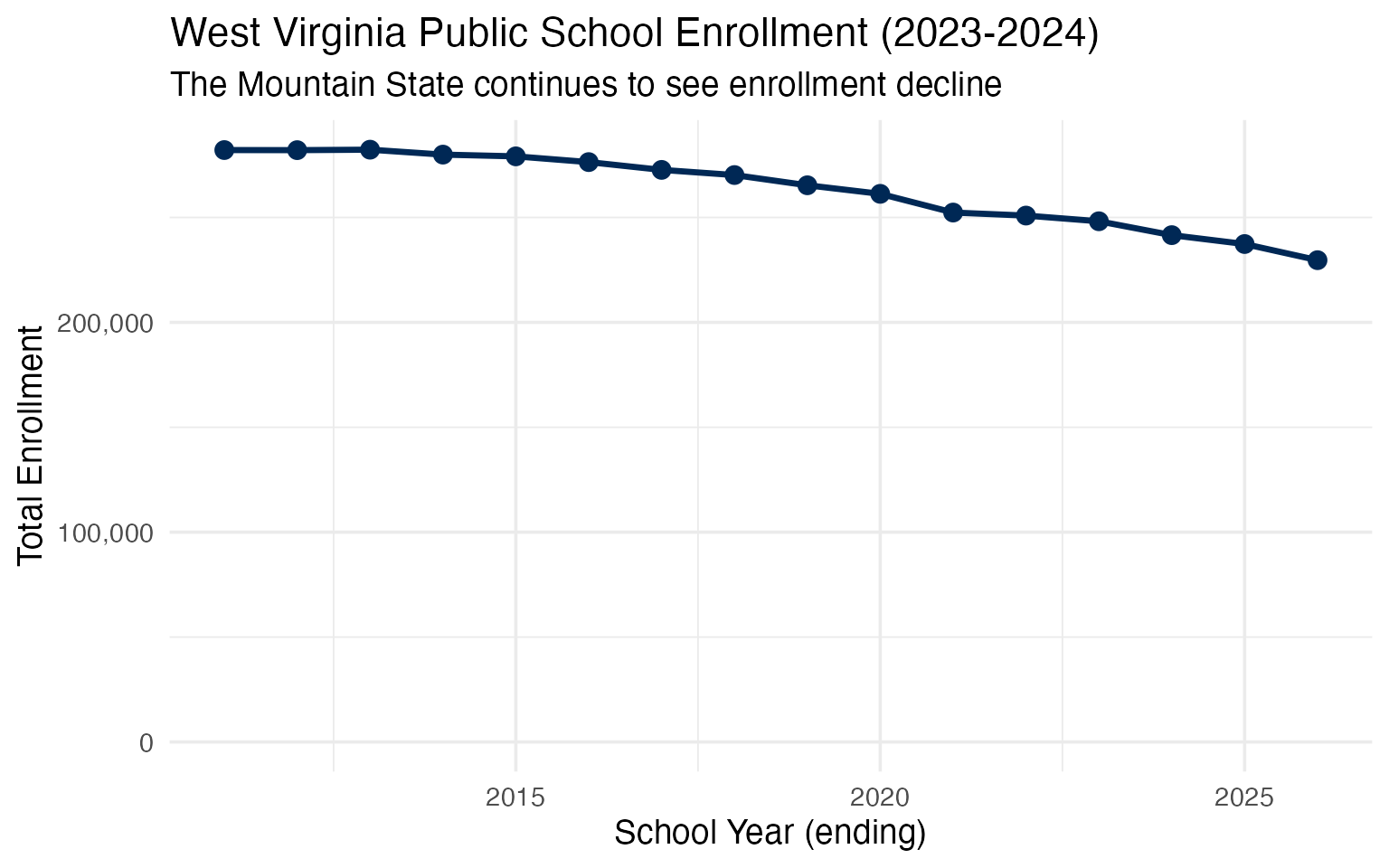
1. West Virginia educates around 250,000 students
West Virginia’s public schools serve roughly a quarter million students across 55 county-based school districts – one of the simplest administrative structures in the nation.
# Get available years (2023-2024)
available_years <- get_available_years()
enr <- fetch_enr_multi(available_years, use_cache = TRUE)

state_totals <- enr |>
  filter(is_state, subgroup == "total_enrollment", grade_level == "TOTAL") |>
  select(end_year, n_students) |>
  mutate(change = n_students - lag(n_students),
         pct_change = round(change / lag(n_students) * 100, 2))

state_totals
#>    end_year n_students change pct_change
#> 1      2011     282130     NA         NA
#> 2      2012     282088    -42      -0.01
#> 3      2013     282309    221       0.08
#> 4      2014     279960  -2349      -0.83
#> 5      2015     279133   -827      -0.30
#> 6      2016     276391  -2742      -0.98
#> 7      2017     272681  -3710      -1.34
#> 8      2018     270220  -2461      -0.90
#> 9      2019     265344  -4876      -1.80
#> 10     2020     261264  -4080      -1.54
#> 11     2021     252346  -8918      -3.41
#> 12     2022     250899  -1447      -0.57
#> 13     2023     248191  -2708      -1.08
#> 14     2024     241574  -6617      -2.67
#> 15     2025     237339  -4235      -1.75
#> 16     2026     229646  -7693      -3.24
ggplot(state_totals, aes(x = end_year, y = n_students)) +
  geom_line(linewidth = 1.2, color = "#002855") +
  geom_point(size = 3, color = "#002855") +
  scale_y_continuous(labels = scales::comma,
                     limits = c(0, NA)) +
  labs(
    title = "West Virginia Public School Enrollment (2023-2024)",
    subtitle = "The Mountain State continues to see enrollment decline",
    x = "School Year (ending)",
    y = "Total Enrollment"
  )
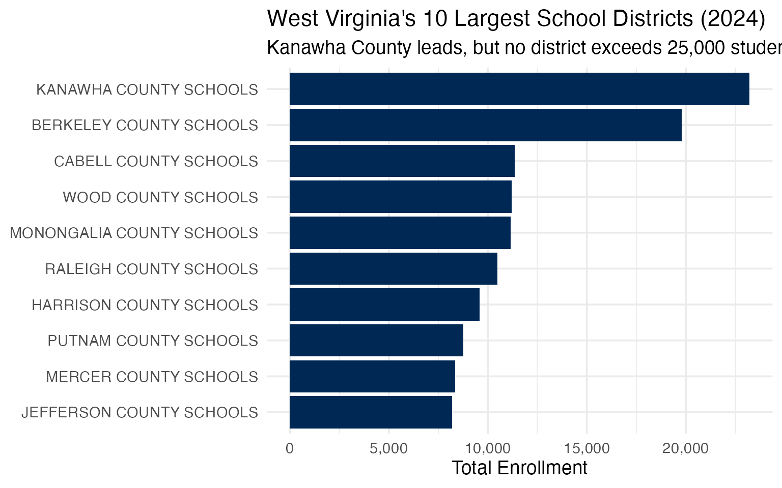
2. Kanawha County is the largest district
Kanawha County, home to the state capital Charleston, is West Virginia’s largest school district – though even it would be considered mid-sized in many states.
enr_2024 <- fetch_enr(2024, use_cache = TRUE)

top_10 <- enr_2024 |>
  filter(is_district, subgroup == "total_enrollment", grade_level == "TOTAL") |>
  arrange(desc(n_students)) |>
  head(10) |>
  select(district_name, county, n_students)

top_10
#>                district_name     county n_students
#> 1     KANAWHA COUNTY SCHOOLS    KANAWHA      23219
#> 2    BERKELEY COUNTY SCHOOLS   BERKELEY      19785
#> 3      CABELL COUNTY SCHOOLS     CABELL      11365
#> 4        WOOD COUNTY SCHOOLS       WOOD      11215
#> 5  MONONGALIA COUNTY SCHOOLS MONONGALIA      11159
#> 6     RALEIGH COUNTY SCHOOLS    RALEIGH      10494
#> 7    HARRISON COUNTY SCHOOLS   HARRISON       9572
#> 8      PUTNAM COUNTY SCHOOLS     PUTNAM       8764
#> 9      MERCER COUNTY SCHOOLS     MERCER       8354
#> 10  JEFFERSON COUNTY SCHOOLS  JEFFERSON       8181
top_10 |>
  mutate(district_name = forcats::fct_reorder(district_name, n_students)) |>
  ggplot(aes(x = n_students, y = district_name)) +
  geom_col(fill = "#002855") +
  scale_x_continuous(labels = scales::comma) +
  labs(
    title = "West Virginia's 10 Largest School Districts (2024)",
    subtitle = "Kanawha County leads, but no district exceeds 25,000 students",
    x = "Total Enrollment",
    y = NULL
  )
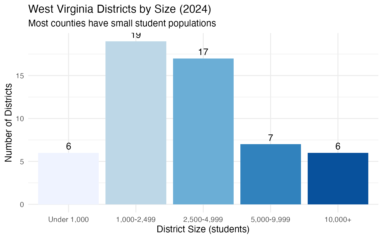
3. Small counties dominate the landscape
West Virginia’s county-based system means many very small districts. Several counties have fewer than 1,000 students total.
# Analyze district size distribution
size_distribution <- enr_2024 |>
  filter(is_district, subgroup == "total_enrollment", grade_level == "TOTAL") |>
  mutate(size_category = case_when(
    n_students < 1000 ~ "Under 1,000",
    n_students < 2500 ~ "1,000-2,499",
    n_students < 5000 ~ "2,500-4,999",
    n_students < 10000 ~ "5,000-9,999",
    TRUE ~ "10,000+"
  )) |>
  mutate(size_category = factor(size_category,
                                 levels = c("Under 1,000", "1,000-2,499",
                                           "2,500-4,999", "5,000-9,999", "10,000+"))) |>
  group_by(size_category) |>
  summarize(
    n_districts = n(),
    total_students = sum(n_students, na.rm = TRUE),
    .groups = "drop"
  )

size_distribution
#> # A tibble: 5 x 3
#>   size_category n_districts total_students
#>   <fct>               <int>          <dbl>
#> 1 Under 1,000             6           5175
#> 2 1,000-2,499            19          32609
#> 3 2,500-4,999            17          63011
#> 4 5,000-9,999             7          53542
#> 5 10,000+                 6          87237
size_distribution |>
  ggplot(aes(x = size_category, y = n_districts, fill = size_category)) +
  geom_col(show.legend = FALSE) +
  geom_text(aes(label = n_districts), vjust = -0.5) +
  scale_fill_brewer(palette = "Blues") +
  labs(
    title = "West Virginia Districts by Size (2024)",
    subtitle = "Most counties have small student populations",
    x = "District Size (students)",
    y = "Number of Districts"
  )
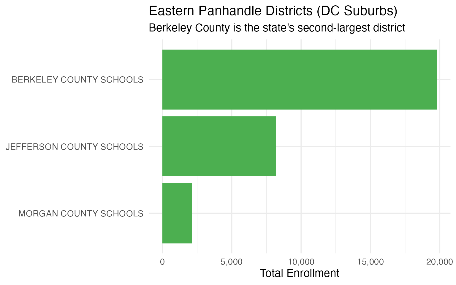
4. The Eastern Panhandle has the largest suburban districts
The Eastern Panhandle – Berkeley, Jefferson, and Morgan counties near Washington, D.C. – benefits from suburban spillover and has some of the state’s fastest-growing areas.
# Eastern Panhandle counties (DC suburbs)
panhandle <- c("BERKELEY", "JEFFERSON", "MORGAN")

regional_comparison <- enr_2024 |>
  filter(is_district, subgroup == "total_enrollment", grade_level == "TOTAL") |>
  mutate(region = case_when(
    county %in% panhandle ~ "Eastern Panhandle",
    TRUE ~ "Rest of State"
  )) |>
  group_by(region) |>
  summarize(
    n_districts = n(),
    total_students = sum(n_students, na.rm = TRUE),
    avg_district_size = round(mean(n_students), 0),
    .groups = "drop"
  )

regional_comparison
#> # A tibble: 2 x 4
#>   region            n_districts total_students avg_district_size
#>   <chr>                   <int>          <dbl>             <dbl>
#> 1 Eastern Panhandle           3          30094             10031
#> 2 Rest of State              52         211480              4067
panhandle_districts <- enr_2024 |>
  filter(is_district, county %in% panhandle,
         subgroup == "total_enrollment", grade_level == "TOTAL") |>
  select(district_name, county, n_students)

panhandle_districts |>
  mutate(district_name = forcats::fct_reorder(district_name, n_students)) |>
  ggplot(aes(x = n_students, y = district_name)) +
  geom_col(fill = "#4CAF50") +
  scale_x_continuous(labels = scales::comma) +
  labs(
    title = "Eastern Panhandle Districts (DC Suburbs)",
    subtitle = "Berkeley County is the state's second-largest district",
    x = "Total Enrollment",
    y = NULL
  )
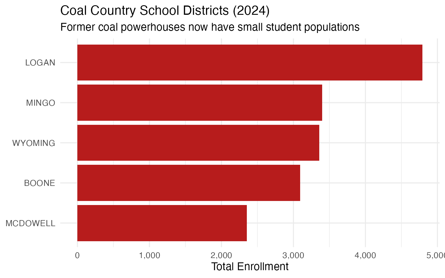
5. Coal country has the smallest districts
The southern coalfield counties – McDowell, Wyoming, Mingo, Logan, and Boone – have experienced decades of population loss as the coal industry contracted.
# Coal counties
coal_counties <- c("MCDOWELL", "WYOMING", "MINGO", "LOGAN", "BOONE")

coal_districts <- enr_2024 |>
  filter(is_district, county %in% coal_counties,
         subgroup == "total_enrollment", grade_level == "TOTAL") |>
  select(district_name, county, n_students) |>
  arrange(n_students)

coal_districts
#>             district_name   county n_students
#> 1 MCDOWELL COUNTY SCHOOLS MCDOWELL       2352
#> 2    BOONE COUNTY SCHOOLS    BOONE       3092
#> 3  WYOMING COUNTY SCHOOLS  WYOMING       3360
#> 4    MINGO COUNTY SCHOOLS    MINGO       3400
#> 5    LOGAN COUNTY SCHOOLS    LOGAN       4791
coal_districts |>
  mutate(county = forcats::fct_reorder(county, n_students)) |>
  ggplot(aes(x = n_students, y = county)) +
  geom_col(fill = "#B71C1C") +
  scale_x_continuous(labels = scales::comma) +
  labs(
    title = "Coal Country School Districts (2024)",
    subtitle = "Former coal powerhouses now have small student populations",
    x = "Total Enrollment",
    y = NULL
  )
6. McDowell County exemplifies Appalachian decline
McDowell County, once a coal mining powerhouse with over 100,000 residents in 1950, now has fewer than 2,500 students – one of the starkest examples of Appalachian population decline.
mcdowell <- enr |>
  filter(is_district, county == "MCDOWELL",
         subgroup == "total_enrollment", grade_level == "TOTAL") |>
  select(end_year, n_students)

mcdowell
#>    end_year n_students
#> 1      2011       3559
#> 2      2012       3535
#> 3      2013       3537
#> 4      2014       3436
#> 5      2015       3417
#> 6      2016       3296
#> 7      2017       3200
#> 8      2018       3056
#> 9      2019       2967
#> 10     2020       2824
#> 11     2021       2637
#> 12     2022       2551
#> 13     2023       2454
#> 14     2024       2352
#> 15     2025       2236
#> 16     2026       2075
7. High school enrollment patterns
Analyzing enrollment by grade level reveals the pipeline of students moving through the system.
grade_trends <- enr_2024 |>
  filter(is_state, subgroup == "total_enrollment",
         grade_level %in% c("K", "05", "09", "12")) |>
  select(grade_level, n_students)

grade_trends
#>   grade_level n_students
#> 1           K      16473
#> 2          05      17791
#> 3          09      20379
#> 4          12      16405
8. Berkeley County is the fastest-growing region
Berkeley County in the Eastern Panhandle is West Virginia’s second-largest district and one of its few growing areas.
# Compare Berkeley to state average
berkeley <- enr_2024 |>
  filter(is_district, county == "BERKELEY",
         subgroup == "total_enrollment", grade_level == "TOTAL") |>
  select(district_name, n_students)

state_avg <- enr_2024 |>
  filter(is_district, subgroup == "total_enrollment", grade_level == "TOTAL") |>
  summarize(avg_enrollment = mean(n_students, na.rm = TRUE))

cat("Berkeley County enrollment:", berkeley$n_students, "\n")
#> Berkeley County enrollment: 19785
cat("State average district enrollment:", round(state_avg$avg_enrollment, 0), "\n")
#> State average district enrollment: 4392
cat("Berkeley is", round(berkeley$n_students / state_avg$avg_enrollment, 1), "x the state average\n")
#> Berkeley is 4.5 x the state average
9. Kindergarten enrollment signals future trends
Kindergarten enrollment serves as a leading indicator. Current K enrollment suggests what high school classes will look like in 12 years.
k_enrollment <- enr_2024 |>
  filter(is_state, subgroup == "total_enrollment", grade_level == "K") |>
  pull(n_students)

grade12_enrollment <- enr_2024 |>
  filter(is_state, subgroup == "total_enrollment", grade_level == "12") |>
  pull(n_students)

cat("Current Kindergarten enrollment:", format(k_enrollment, big.mark = ","), "\n")
#> Current Kindergarten enrollment: 16,473
cat("Current 12th grade enrollment:", format(grade12_enrollment, big.mark = ","), "\n")
#> Current 12th grade enrollment: 16,405
cat("K is", round((k_enrollment/grade12_enrollment - 1) * 100, 1), "% different from 12th grade\n")
#> K is 0.4 % different from 12th grade
10. 55 districts create administrative structure
West Virginia’s county-based system means even tiny counties maintain full district operations. Several counties have student populations smaller than individual schools in other states.
smallest <- enr_2024 |>
  filter(is_district, subgroup == "total_enrollment", grade_level == "TOTAL") |>
  arrange(n_students) |>
  head(10) |>
  select(district_name, county, n_students)

smallest
#>                district_name     county n_students
#> 1      GILMER COUNTY SCHOOLS     GILMER        761
#> 2     CALHOUN COUNTY SCHOOLS    CALHOUN        821
#> 3   PENDLETON COUNTY SCHOOLS  PENDLETON        843
#> 4        WIRT COUNTY SCHOOLS       WIRT        894
#> 5  POCAHONTAS COUNTY SCHOOLS POCAHONTAS        915
#> 6      TUCKER COUNTY SCHOOLS     TUCKER        941
#> 7   PLEASANTS COUNTY SCHOOLS  PLEASANTS       1051
#> 8     WEBSTER COUNTY SCHOOLS    WEBSTER       1116
#> 9   DODDRIDGE COUNTY SCHOOLS  DODDRIDGE       1142
#> 10    RITCHIE COUNTY SCHOOLS    RITCHIE       1144
Counties like Wirt, Calhoun, and Pocahontas each maintain a full school district despite having fewer students than many individual elementary schools elsewhere.
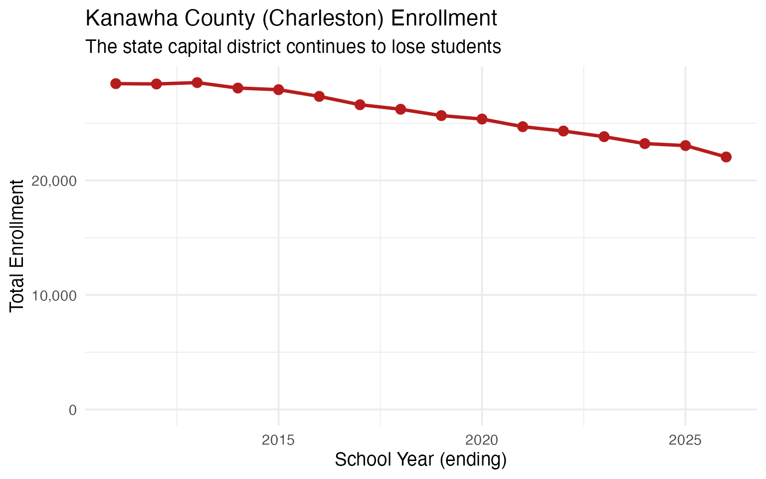
11. Kanawha County (Charleston) is the state capital’s district
The state capital Charleston, in Kanawha County, is West Virginia’s largest school district with over 23,000 students.
kanawha <- enr |>
  filter(is_district, county == "KANAWHA",
         subgroup == "total_enrollment", grade_level == "TOTAL") |>
  select(end_year, n_students)

kanawha
#>    end_year n_students
#> 1      2011      28458
#> 2      2012      28429
#> 3      2013      28548
#> 4      2014      28072
#> 5      2015      27931
#> 6      2016      27345
#> 7      2017      26615
#> 8      2018      26221
#> 9      2019      25666
#> 10     2020      25365
#> 11     2021      24698
#> 12     2022      24318
#> 13     2023      23826
#> 14     2024      23219
#> 15     2025      23048
#> 16     2026      22051
ggplot(kanawha, aes(x = end_year, y = n_students)) +
  geom_line(linewidth = 1.2, color = "#B71C1C") +
  geom_point(size = 3, color = "#B71C1C") +
  scale_y_continuous(labels = scales::comma, limits = c(0, NA)) +
  labs(
    title = "Kanawha County (Charleston) Enrollment",
    subtitle = "The state capital district continues to lose students",
    x = "School Year (ending)",
    y = "Total Enrollment"
  )
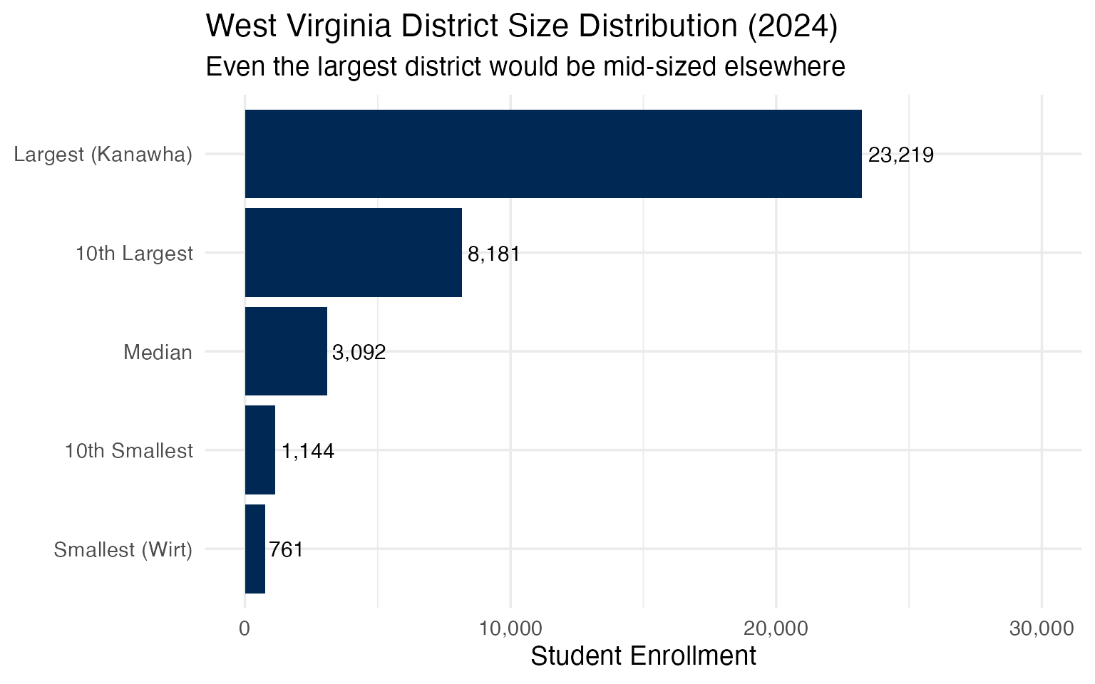
12. The urban-rural divide is minimal
West Virginia has no large cities. Even “urban” Kanawha County is mostly rural by national standards. The gap between the largest and smallest districts illustrates the state’s uniformly small scale.
district_sizes <- enr_2024 |>
  filter(is_district, subgroup == "total_enrollment", grade_level == "TOTAL") |>
  arrange(desc(n_students)) |>
  mutate(rank = row_number()) |>
  select(rank, district_name, county, n_students)

size_range <- tibble(
  metric = c("Largest (Kanawha)", "10th Largest", "Median", "10th Smallest", "Smallest (Wirt)"),
  n_students = c(
    district_sizes$n_students[1],
    district_sizes$n_students[10],
    median(district_sizes$n_students),
    district_sizes$n_students[46],
    district_sizes$n_students[55]
  )
)

size_range
#> # A tibble: 5 x 2
#>   metric            n_students
#>   <chr>                  <dbl>
#> 1 Largest (Kanawha)      23219
#> 2 10th Largest            8181
#> 3 Median                  3092
#> 4 10th Smallest           1144
#> 5 Smallest (Wirt)          761
size_range |>
  mutate(metric = factor(metric, levels = rev(metric))) |>
  ggplot(aes(x = n_students, y = metric)) +
  geom_col(fill = "#002855") +
  geom_text(aes(label = scales::comma(n_students)), hjust = -0.1, size = 4) +
  scale_x_continuous(labels = scales::comma, limits = c(0, 30000)) +
  labs(
    title = "West Virginia District Size Distribution (2024)",
    subtitle = "Even the largest district would be mid-sized elsewhere",
    x = "Student Enrollment",
    y = NULL
  )
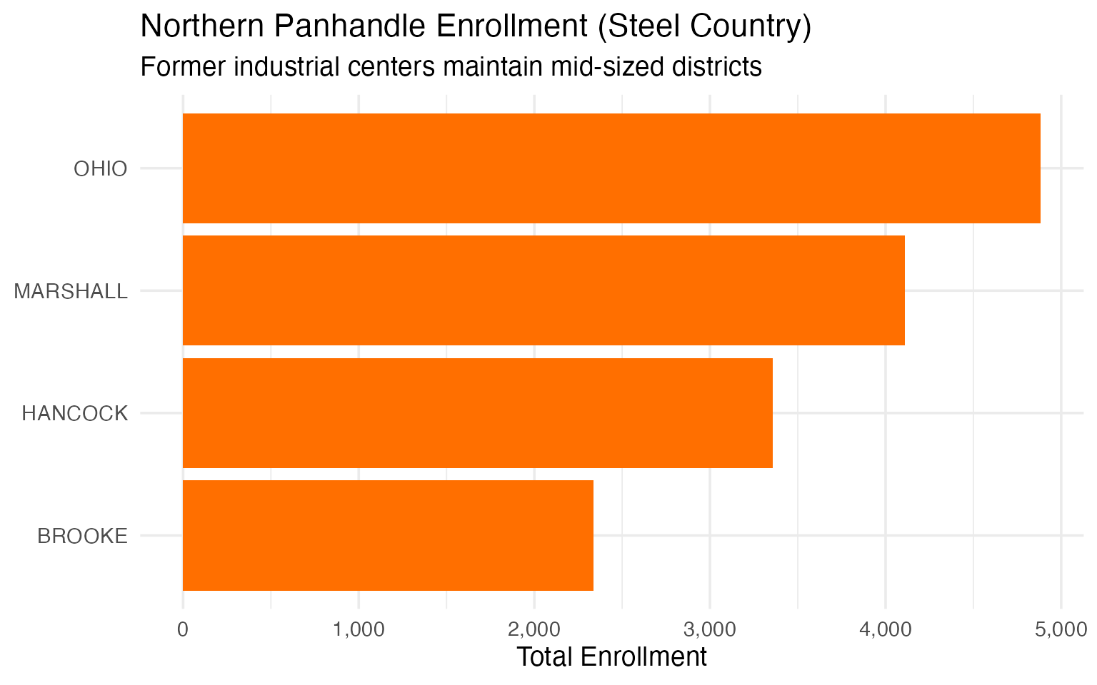
13. The Northern Panhandle steel town legacy
The Northern Panhandle – Ohio, Marshall, Brooke, and Hancock counties – once thrived on steel and manufacturing. These communities now have small to mid-sized districts.
northern_panhandle <- c("OHIO", "MARSHALL", "BROOKE", "HANCOCK")

northern_districts <- enr_2024 |>
  filter(is_district, county %in% northern_panhandle,
         subgroup == "total_enrollment", grade_level == "TOTAL") |>
  select(district_name, county, n_students) |>
  arrange(desc(n_students))

northern_districts
#>             district_name   county n_students
#> 1     OHIO COUNTY SCHOOLS     OHIO       4884
#> 2 MARSHALL COUNTY SCHOOLS MARSHALL       4109
#> 3  HANCOCK COUNTY SCHOOLS  HANCOCK       3356
#> 4   BROOKE COUNTY SCHOOLS   BROOKE       2336
northern_districts |>
  mutate(county = forcats::fct_reorder(county, n_students)) |>
  ggplot(aes(x = n_students, y = county)) +
  geom_col(fill = "#FF6F00") +
  scale_x_continuous(labels = scales::comma) +
  labs(
    title = "Northern Panhandle Enrollment (Steel Country)",
    subtitle = "Former industrial centers maintain mid-sized districts",
    x = "Total Enrollment",
    y = NULL
  )
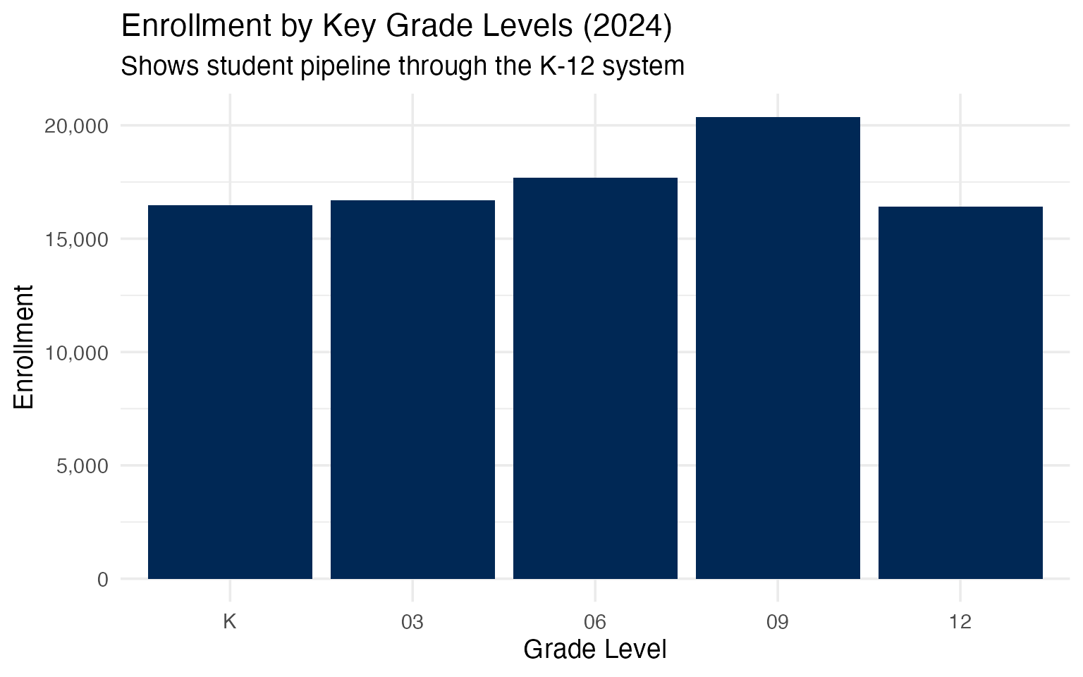
14. Grade-level enrollment by benchmark grades
Comparing enrollment across key grade levels (K, 3, 6, 9, 12) shows the flow of students through the system.
grade_comparison <- enr_2024 |>
  filter(is_state, subgroup == "total_enrollment",
         grade_level %in% c("K", "03", "06", "09", "12")) |>
  select(grade_level, n_students) |>
  mutate(grade_level = factor(grade_level, levels = c("K", "03", "06", "09", "12")))

grade_comparison
#>   grade_level n_students
#> 1           K      16473
#> 2          03      16683
#> 3          06      17683
#> 4          09      20379
#> 5          12      16405
ggplot(grade_comparison, aes(x = grade_level, y = n_students)) +
  geom_col(fill = "#002855") +
  scale_y_continuous(labels = scales::comma) +
  labs(
    title = "Enrollment by Key Grade Levels (2024)",
    subtitle = "Shows student pipeline through the K-12 system",
    x = "Grade Level",
    y = "Enrollment"
  )
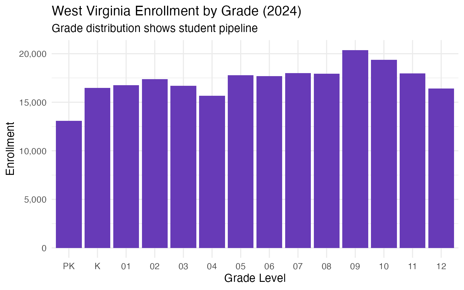
15. The future is written in demographics
West Virginia’s birth rate has declined steadily, reflected in smaller kindergarten cohorts entering the system each year.
# Compare K to total to show pipeline
k_data <- enr_2024 |>
  filter(is_state, subgroup == "total_enrollment", grade_level == "K") |>
  select(n_students) |>
  mutate(grade = "Kindergarten")

total_data <- enr_2024 |>
  filter(is_state, subgroup == "total_enrollment", grade_level == "TOTAL") |>
  select(n_students) |>
  mutate(grade = "All Grades")

k_pct_of_total <- k_data$n_students / total_data$n_students * 100

cat("Kindergarten enrollment:", format(k_data$n_students, big.mark = ","), "\n")
#> Kindergarten enrollment: 16,473
cat("Total enrollment:", format(total_data$n_students, big.mark = ","), "\n")
#> Total enrollment: 241,574
cat("Kindergarten is", round(k_pct_of_total, 1), "% of total enrollment\n")
#> Kindergarten is 6.8 % of total enrollment
# Show all grade levels
all_grades <- enr_2024 |>
  filter(is_state, subgroup == "total_enrollment",
         grade_level %in% c("PK", "K", "01", "02", "03", "04", "05",
                           "06", "07", "08", "09", "10", "11", "12")) |>
  select(grade_level, n_students) |>
  mutate(grade_level = factor(grade_level,
                              levels = c("PK", "K", "01", "02", "03", "04", "05",
                                        "06", "07", "08", "09", "10", "11", "12")))

ggplot(all_grades, aes(x = grade_level, y = n_students)) +
  geom_col(fill = "#673AB7") +
  scale_y_continuous(labels = scales::comma) +
  labs(
    title = "West Virginia Enrollment by Grade (2024)",
    subtitle = "Grade distribution shows student pipeline",
    x = "Grade Level",
    y = "Enrollment"
  )
Summary
West Virginia’s school enrollment data reveals: - Quarter million students: ~250,000 students across 55 county school districts - Uniform small scale: Even the largest district (Kanawha) has only ~23,000 students - Eastern Panhandle exception: DC suburb spillover creates growth areas - Coal country decline: Southern counties have the smallest enrollments - Simple structure: One district per county, mandated by the state constitution
These patterns reflect broader demographic and economic forces reshaping Appalachia.
Data sourced from West Virginia Department of Education (WVDE) School Finance Data.
Session Info
sessionInfo()
#> R version 4.5.0 (2025-04-11)
#> Platform: aarch64-apple-darwin22.6.0
#> Running under: macOS 26.1
#>
#> Matrix products: default
#> BLAS:   /opt/homebrew/Cellar/openblas/0.3.30/lib/libopenblasp-r0.3.30.dylib
#> LAPACK: /opt/homebrew/Cellar/r/4.5.0/lib/R/lib/libRlapack.dylib;  LAPACK version 3.12.1
#>
#> locale:
#> [1] C.UTF-8/C.UTF-8/C.UTF-8/C/C.UTF-8/C.UTF-8
#>
#> time zone: America/New_York
#> tzcode source: internal
#>
#> attached base packages:
#> [1] stats     graphics  grDevices utils     datasets  methods   base
#>
#> other attached packages:
#> [1] ggplot2_4.0.1      tidyr_1.3.2        dplyr_1.2.0        wvschooldata_0.2.0
#>
#> loaded via a namespace (and not attached):
#>  [1] utf8_1.2.6         rappdirs_0.3.4     sass_0.4.10        generics_0.1.4
#>  [5] digest_0.6.39      magrittr_2.0.4     evaluate_1.0.5     grid_4.5.0
#>  [9] RColorBrewer_1.1-3 fastmap_1.2.0      cellranger_1.1.0   jsonlite_2.0.0
#> [13] httr_1.4.8         purrr_1.2.1        scales_1.4.0       codetools_0.2-20
#> [17] textshaping_1.0.4  jquerylib_0.1.4    cli_3.6.5          pdftools_3.7.0
#> [21] rlang_1.1.7        withr_3.0.2        cachem_1.1.0       yaml_2.3.12
#> [25] otel_0.2.0         tools_4.5.0        forcats_1.0.1      curl_7.0.0
#> [29] vctrs_0.7.1        R6_2.6.1           lifecycle_1.0.5    fs_1.6.6
#> [33] htmlwidgets_1.6.4  ragg_1.5.0         pkgconfig_2.0.3    desc_1.4.3
#> [37] pkgdown_2.2.0      pillar_1.11.1      bslib_0.9.0        gtable_0.3.6
#> [41] glue_1.8.0         Rcpp_1.1.1         systemfonts_1.3.1  xfun_0.55
#> [45] tibble_3.3.1       tidyselect_1.2.1   knitr_1.51         farver_2.1.2
#> [49] htmltools_0.5.9    rmarkdown_2.30     labeling_0.4.3     qpdf_1.4.1
#> [53] compiler_4.5.0     S7_0.2.1           askpass_1.2.1      readxl_1.4.5