15 Insights from Florida Assessment Data
Source:vignettes/florida-assessment.Rmd
florida-assessment.Rmd
library(flschooldata)
library(dplyr)
library(tidyr)
library(ggplot2)

theme_set(theme_minimal(base_size = 14))
This vignette explores Florida’s assessment data from the FAST (Florida Assessment of Student Thinking) and FSA (Florida Standards Assessments) programs, covering grades 3-10 in ELA and grades 3-8 in Mathematics.
Assessment Systems: - FSA (Florida Standards Assessments): 2015-2022 - FAST (Florida Assessment of Student Thinking): 2023-present
Achievement Levels: - Level 1: Inadequate - Level 2: Below Satisfactory - Level 3: Satisfactory - Level 4: Proficient - Level 5: Mastery
Students at Level 3 or above are considered “on grade level” or proficient.
1. Just over half of Florida third graders read on grade level
In 2024, 55% of Florida 3rd graders scored at Level 3 or above on the FAST ELA Reading assessment.
assess_2024 <- fetch_assessment(2024, "ela", grade = 3, level = "district",
                                 tidy = FALSE, use_cache = TRUE)

state_g3 <- assess_2024 |>
  filter(is_state) |>
  select(end_year, subject, grade, n_tested, pct_proficient,
         pct_level_1, pct_level_2, pct_level_3, pct_level_4, pct_level_5)

state_g3
#> # A tibble: 1 × 10
#>   end_year subject grade n_tested pct_proficient pct_level_1 pct_level_2
#>      <dbl> <chr>   <chr>    <dbl>          <dbl>       <dbl>       <dbl>
#> 1     2024 ELA     03      216473             55          22          22
#> # ℹ 3 more variables: pct_level_3 <dbl>, pct_level_4 <dbl>, pct_level_5 <dbl>
stopifnot(nrow(state_g3) > 0)
levels_long <- state_g3 |>
  pivot_longer(cols = starts_with("pct_level"),
               names_to = "level",
               values_to = "pct") |>
  mutate(level = gsub("pct_level_", "Level ", level),
         level = factor(level, levels = paste("Level", 1:5)))

ggplot(levels_long, aes(x = level, y = pct, fill = level)) +
  geom_col() +
  geom_text(aes(label = paste0(pct, "%")), vjust = -0.3) +
  scale_fill_manual(values = c("#D7191C", "#FDAE61", "#FFFFBF", "#A6D96A", "#1A9641")) +
  labs(
    title = "Florida 3rd Grade ELA Achievement Levels (2024)",
    subtitle = "55% scored at Level 3 or above (proficient)",
    x = "Achievement Level",
    y = "Percent of Students"
  ) +
  theme(legend.position = "none")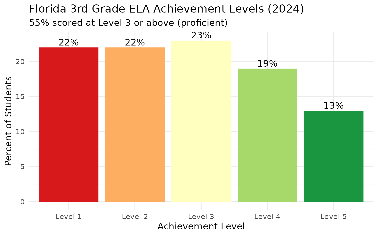
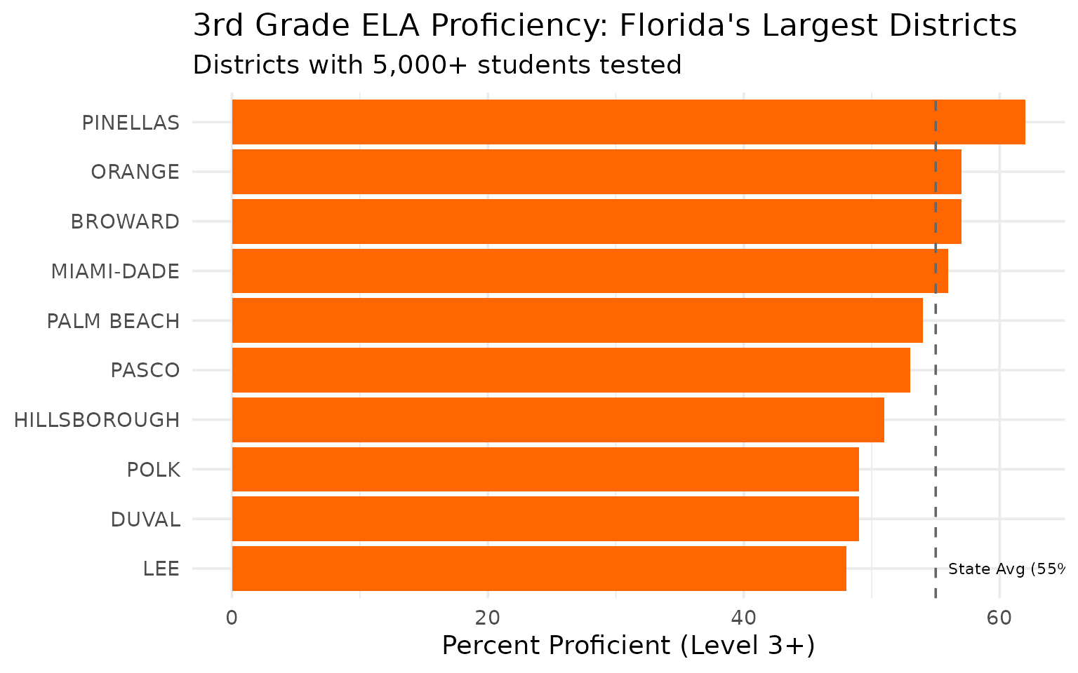
2. Miami-Dade outperforms the state average
Despite being the largest district with over 25,000 3rd graders tested, Miami-Dade’s 56% proficiency rate exceeds the state average.
large_districts <- assess_2024 |>
  filter(!is_state, n_tested > 5000) |>
  arrange(desc(n_tested)) |>
  select(district_name, n_tested, pct_proficient) |>
  head(10)

large_districts
#> # A tibble: 10 × 3
#>    district_name n_tested pct_proficient
#>    <chr>            <dbl>          <dbl>
#>  1 MIAMI-DADE       25178             56
#>  2 BROWARD          18457             57
#>  3 HILLSBOROUGH     16802             51
#>  4 ORANGE           15743             57
#>  5 PALM BEACH       14593             54
#>  6 DUVAL            10095             49
#>  7 POLK              9295             49
#>  8 LEE               7644             48
#>  9 PINELLAS          6654             62
#> 10 PASCO             6511             53
stopifnot(nrow(large_districts) > 0)
large_districts |>
  mutate(district_name = forcats::fct_reorder(district_name, pct_proficient)) |>
  ggplot(aes(x = pct_proficient, y = district_name)) +
  geom_col(fill = "#FF6600") +
  geom_vline(xintercept = 55, linetype = "dashed", color = "gray40") +
  annotate("text", x = 56, y = 1, label = "State Avg (55%)", hjust = 0, size = 3) +
  labs(
    title = "3rd Grade ELA Proficiency: Florida's Largest Districts",
    subtitle = "Districts with 5,000+ students tested",
    x = "Percent Proficient (Level 3+)",
    y = NULL
  )
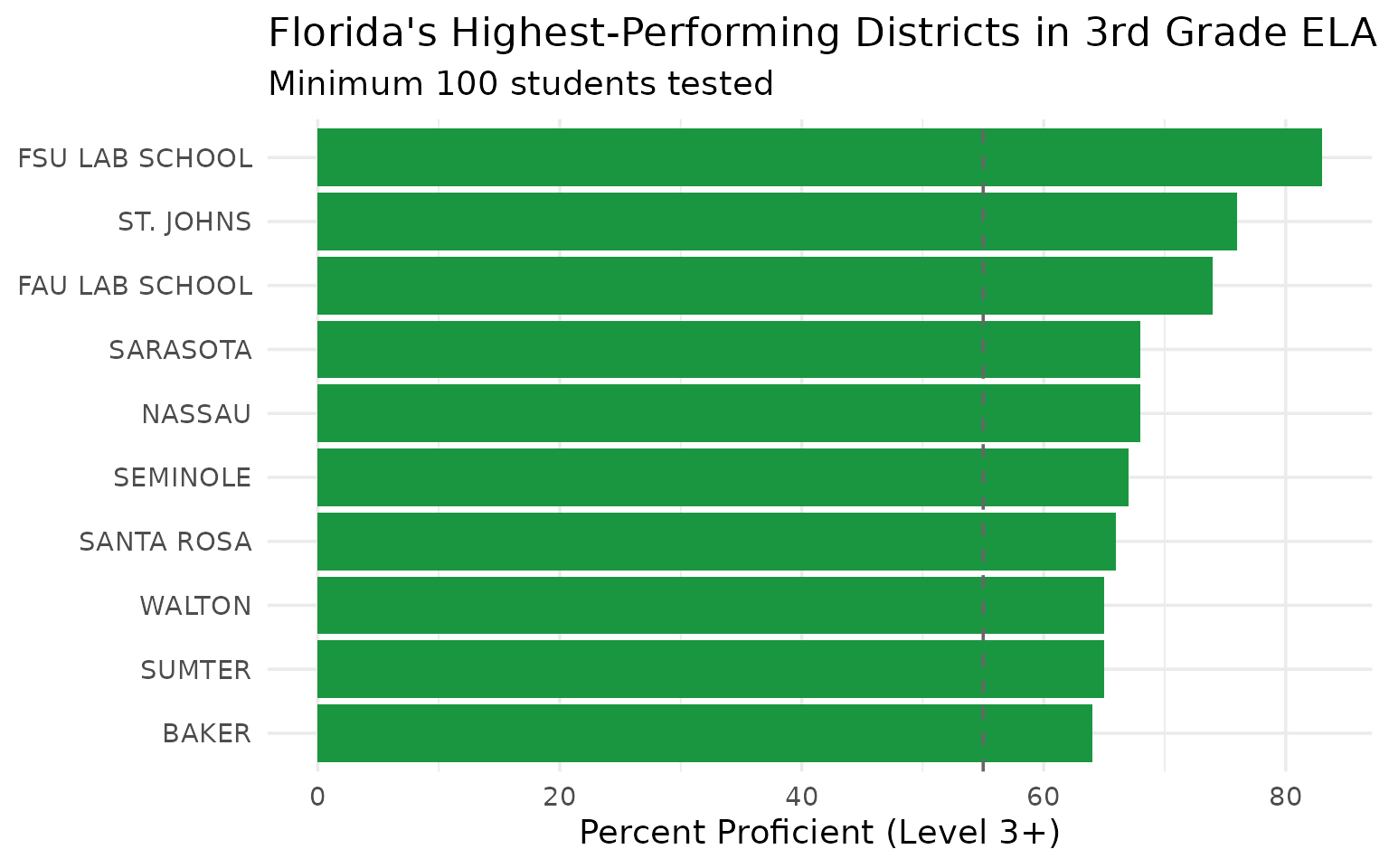
3. Small districts lead in proficiency rates
Several smaller counties have the highest proficiency rates in the state, with some exceeding 70%.
top_proficient <- assess_2024 |>
  filter(!is_state, n_tested >= 100) |>
  arrange(desc(pct_proficient)) |>
  select(district_name, n_tested, pct_proficient) |>
  head(10)

top_proficient
#> # A tibble: 10 × 3
#>    district_name  n_tested pct_proficient
#>    <chr>             <dbl>          <dbl>
#>  1 FSU LAB SCHOOL      238             83
#>  2 ST. JOHNS          3706             76
#>  3 FAU LAB SCHOOL      219             74
#>  4 NASSAU              931             68
#>  5 SARASOTA           3313             68
#>  6 SEMINOLE           4653             67
#>  7 SANTA ROSA         2198             66
#>  8 SUMTER              765             65
#>  9 WALTON              914             65
#> 10 BAKER               373             64
stopifnot(nrow(top_proficient) > 0)
top_proficient |>
  mutate(district_name = forcats::fct_reorder(district_name, pct_proficient)) |>
  ggplot(aes(x = pct_proficient, y = district_name)) +
  geom_col(fill = "#1A9641") +
  geom_vline(xintercept = 55, linetype = "dashed", color = "gray40") +
  labs(
    title = "Florida's Highest-Performing Districts in 3rd Grade ELA",
    subtitle = "Minimum 100 students tested",
    x = "Percent Proficient (Level 3+)",
    y = NULL
  )
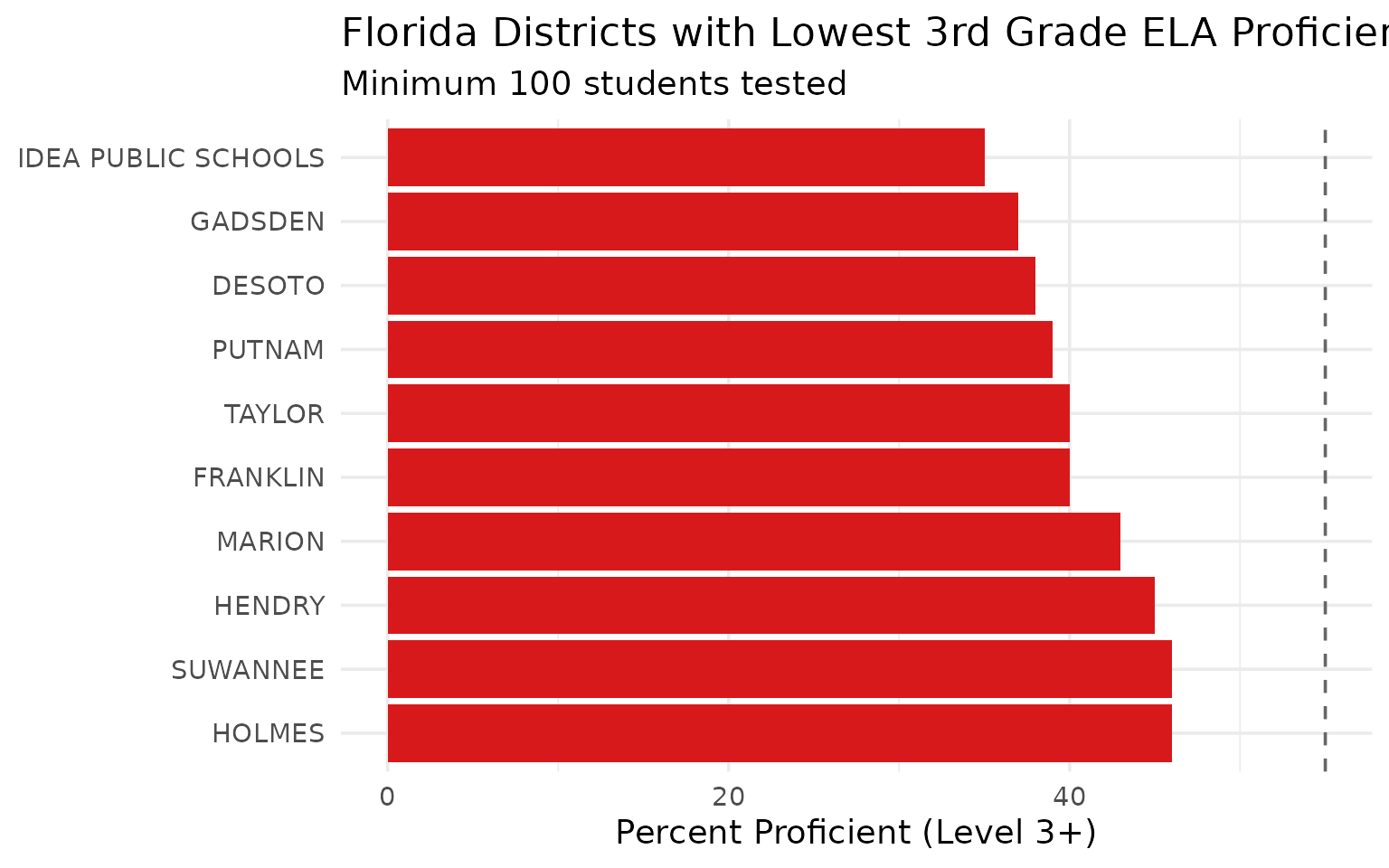
4. Rural Panhandle counties face challenges
Many North Florida rural counties have proficiency rates below 50%.
low_proficient <- assess_2024 |>
  filter(!is_state, n_tested >= 100) |>
  arrange(pct_proficient) |>
  select(district_name, n_tested, pct_proficient) |>
  head(10)

low_proficient
#> # A tibble: 10 × 3
#>    district_name       n_tested pct_proficient
#>    <chr>                  <dbl>          <dbl>
#>  1 IDEA PUBLIC SCHOOLS      395             35
#>  2 GADSDEN                  359             37
#>  3 DESOTO                   351             38
#>  4 PUTNAM                   841             39
#>  5 FRANKLIN                 101             40
#>  6 TAYLOR                   210             40
#>  7 MARION                  3709             43
#>  8 HENDRY                   855             45
#>  9 HOLMES                   233             46
#> 10 SUWANNEE                 450             46
stopifnot(nrow(low_proficient) > 0)
low_proficient |>
  mutate(district_name = forcats::fct_reorder(district_name, -pct_proficient)) |>
  ggplot(aes(x = pct_proficient, y = district_name)) +
  geom_col(fill = "#D7191C") +
  geom_vline(xintercept = 55, linetype = "dashed", color = "gray40") +
  labs(
    title = "Florida Districts with Lowest 3rd Grade ELA Proficiency",
    subtitle = "Minimum 100 students tested",
    x = "Percent Proficient (Level 3+)",
    y = NULL
  )
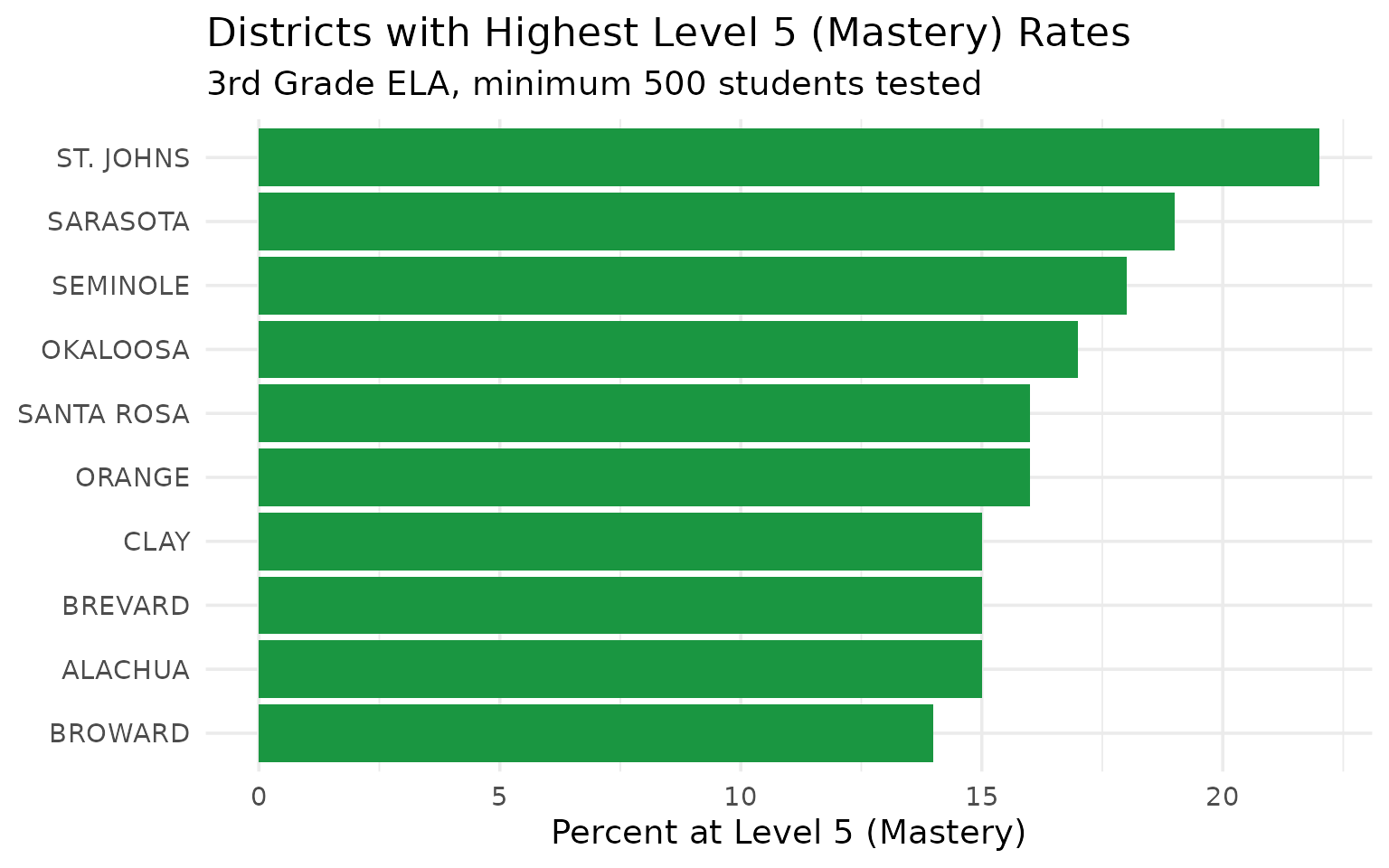
5. Level 5 (Mastery) varies dramatically by district
Some districts have 3x the mastery rate of others.
mastery <- assess_2024 |>
  filter(!is_state, n_tested >= 500) |>
  arrange(desc(pct_level_5)) |>
  select(district_name, n_tested, pct_level_5, pct_proficient) |>
  head(10)

mastery
#> # A tibble: 10 × 4
#>    district_name n_tested pct_level_5 pct_proficient
#>    <chr>            <dbl>       <dbl>          <dbl>
#>  1 ST. JOHNS         3706          22             76
#>  2 SARASOTA          3313          19             68
#>  3 SEMINOLE          4653          18             67
#>  4 OKALOOSA          2516          17             59
#>  5 ORANGE           15743          16             57
#>  6 SANTA ROSA        2198          16             66
#>  7 ALACHUA           2246          15             56
#>  8 BREVARD           5545          15             59
#>  9 CLAY              2978          15             63
#> 10 BROWARD          18457          14             57
stopifnot(nrow(mastery) > 0)
mastery |>
  mutate(district_name = forcats::fct_reorder(district_name, pct_level_5)) |>
  ggplot(aes(x = pct_level_5, y = district_name)) +
  geom_col(fill = "#1A9641") +
  labs(
    title = "Districts with Highest Level 5 (Mastery) Rates",
    subtitle = "3rd Grade ELA, minimum 500 students tested",
    x = "Percent at Level 5 (Mastery)",
    y = NULL
  )
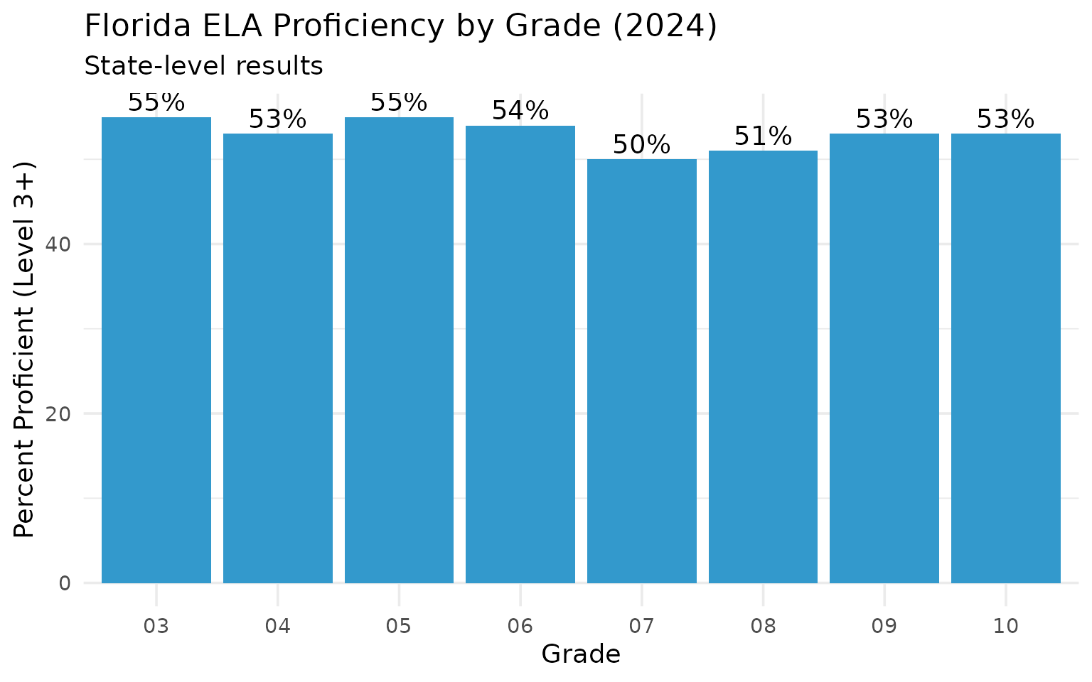
6. Proficiency rises through the grades for ELA
Upper grade students have higher ELA proficiency rates than younger students.
all_grades <- fetch_assessment(2024, "ela", grade = NULL, level = "district",
                                tidy = FALSE, use_cache = TRUE)

grade_state <- all_grades |>
  filter(is_state) |>
  select(grade, n_tested, pct_proficient) |>
  arrange(grade)

grade_state
#> # A tibble: 8 × 3
#>   grade n_tested pct_proficient
#>   <chr>    <dbl>          <dbl>
#> 1 03      216473             55
#> 2 04      213136             53
#> 3 05      204219             55
#> 4 06      205644             54
#> 5 07      215426             50
#> 6 08      210730             51
#> 7 09      217743             53
#> 8 10      217930             53
stopifnot(nrow(grade_state) > 0)
grade_state |>
  ggplot(aes(x = grade, y = pct_proficient)) +
  geom_col(fill = "#3399CC") +
  geom_text(aes(label = paste0(pct_proficient, "%")), vjust = -0.3) +
  labs(
    title = "Florida ELA Proficiency by Grade (2024)",
    subtitle = "State-level results",
    x = "Grade",
    y = "Percent Proficient (Level 3+)"
  )
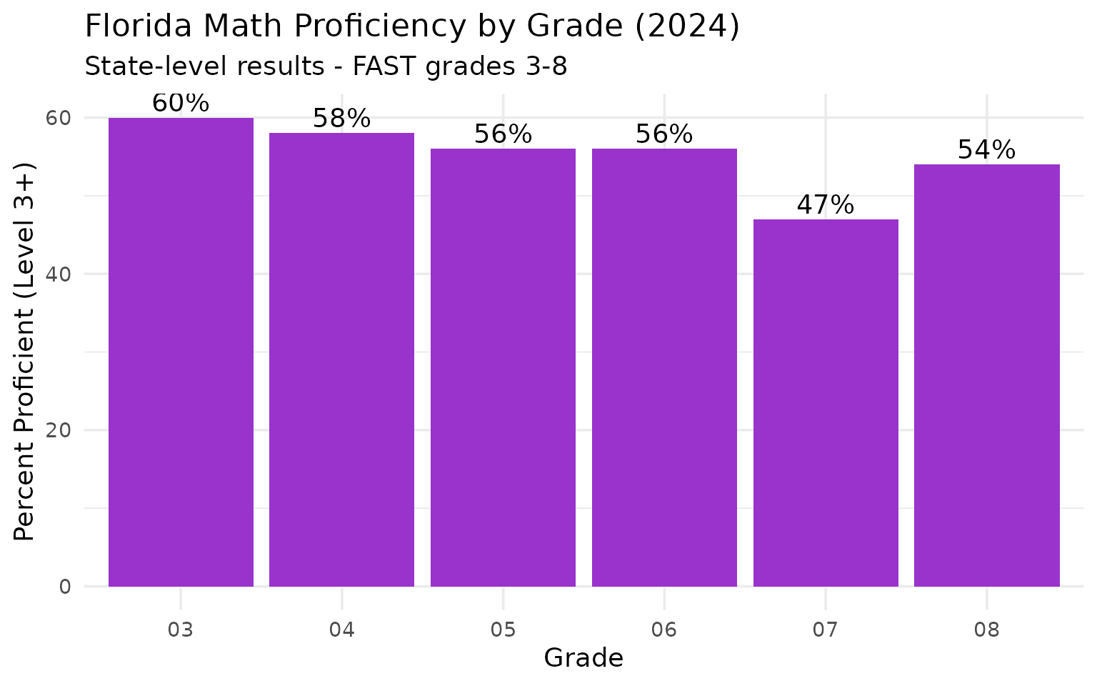
7. Math proficiency peaks in Grade 4
Mathematics proficiency shows a different pattern, with younger grades performing better.
math_all <- fetch_assessment(2024, "math", grade = NULL, level = "district",
                              tidy = FALSE, use_cache = TRUE)

math_state <- math_all |>
  filter(is_state) |>
  select(grade, n_tested, pct_proficient) |>
  arrange(grade)

math_state
#> # A tibble: 6 × 3
#>   grade n_tested pct_proficient
#>   <chr>    <dbl>          <dbl>
#> 1 03      215911             60
#> 2 04      208115             58
#> 3 05      202721             56
#> 4 06      201312             56
#> 5 07      149404             47
#> 6 08      167946             54
stopifnot(nrow(math_state) > 0)
math_state |>
  ggplot(aes(x = grade, y = pct_proficient)) +
  geom_col(fill = "#9933CC") +
  geom_text(aes(label = paste0(pct_proficient, "%")), vjust = -0.3) +
  labs(
    title = "Florida Math Proficiency by Grade (2024)",
    subtitle = "State-level results - FAST grades 3-8",
    x = "Grade",
    y = "Percent Proficient (Level 3+)"
  )
8. Over 216,000 third graders took the ELA assessment
Florida’s massive scale makes even small percentage changes significant in terms of actual students.
counts <- assess_2024 |>
  filter(is_state) |>
  mutate(
    n_proficient = round(pct_proficient / 100 * n_tested),
    n_not_proficient = n_tested - n_proficient
  ) |>
  select(n_tested, n_proficient, n_not_proficient, pct_proficient)

counts
#> # A tibble: 1 × 4
#>   n_tested n_proficient n_not_proficient pct_proficient
#>      <dbl>        <dbl>            <dbl>          <dbl>
#> 1   216473       119060            97413             55
stopifnot(nrow(counts) > 0)
Every 1% change represents over 2,000 students.
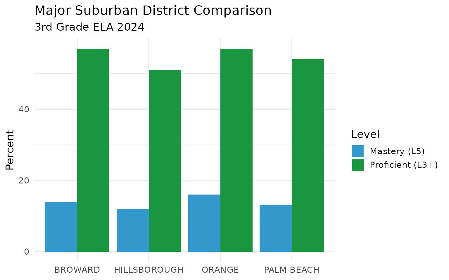
9. Broward edges out Hillsborough
Among large suburban districts, Broward County narrowly outperforms Hillsborough.
suburban <- assess_2024 |>
  filter(district_name %in% c("BROWARD", "HILLSBOROUGH", "ORANGE", "PALM BEACH")) |>
  select(district_name, n_tested, pct_proficient, pct_level_5)

suburban
#> # A tibble: 4 × 4
#>   district_name n_tested pct_proficient pct_level_5
#>   <chr>            <dbl>          <dbl>       <dbl>
#> 1 BROWARD          18457             57          14
#> 2 HILLSBOROUGH     16802             51          12
#> 3 ORANGE           15743             57          16
#> 4 PALM BEACH       14593             54          13
stopifnot(nrow(suburban) > 0)
suburban |>
  pivot_longer(cols = c(pct_proficient, pct_level_5),
               names_to = "metric",
               values_to = "pct") |>
  mutate(metric = ifelse(metric == "pct_proficient", "Proficient (L3+)", "Mastery (L5)")) |>
  ggplot(aes(x = district_name, y = pct, fill = metric)) +
  geom_col(position = "dodge") +
  scale_fill_manual(values = c("#3399CC", "#1A9641")) +
  labs(
    title = "Major Suburban District Comparison",
    subtitle = "3rd Grade ELA 2024",
    x = NULL,
    y = "Percent",
    fill = "Level"
  )
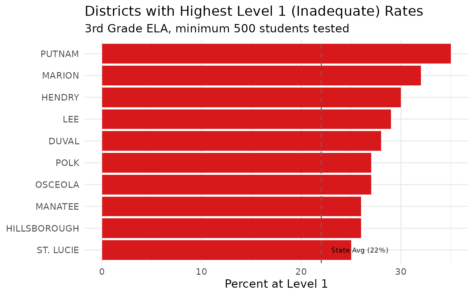
10. Level 1 students need intensive intervention
Statewide, 22% of 3rd graders scored at Level 1 (Inadequate), requiring significant intervention.
level_1 <- assess_2024 |>
  filter(!is_state, n_tested >= 500) |>
  arrange(desc(pct_level_1)) |>
  select(district_name, n_tested, pct_level_1, pct_proficient) |>
  head(10)

level_1
#> # A tibble: 10 × 4
#>    district_name n_tested pct_level_1 pct_proficient
#>    <chr>            <dbl>       <dbl>          <dbl>
#>  1 PUTNAM             841          35             39
#>  2 MARION            3709          32             43
#>  3 HENDRY             855          30             45
#>  4 LEE               7644          29             48
#>  5 DUVAL            10095          28             49
#>  6 OSCEOLA           5442          27             49
#>  7 POLK              9295          27             49
#>  8 HILLSBOROUGH     16802          26             51
#>  9 MANATEE           4358          26             51
#> 10 ST. LUCIE         3410          25             49
stopifnot(nrow(level_1) > 0)
level_1 |>
  mutate(district_name = forcats::fct_reorder(district_name, pct_level_1)) |>
  ggplot(aes(x = pct_level_1, y = district_name)) +
  geom_col(fill = "#D7191C") +
  geom_vline(xintercept = 22, linetype = "dashed", color = "gray40") +
  annotate("text", x = 23, y = 1, label = "State Avg (22%)", hjust = 0, size = 3) +
  labs(
    title = "Districts with Highest Level 1 (Inadequate) Rates",
    subtitle = "3rd Grade ELA, minimum 500 students tested",
    x = "Percent at Level 1",
    y = NULL
  )
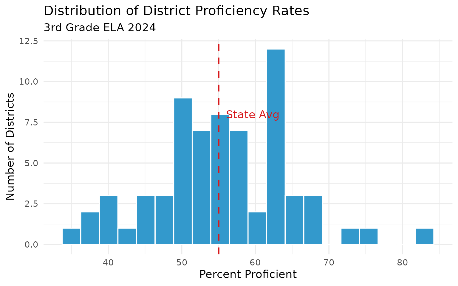
11. The proficiency gap between districts is 40+ percentage points
From top to bottom, Florida districts vary by over 40 percentage points in proficiency.
gap <- assess_2024 |>
  filter(!is_state, n_tested >= 100) |>
  summarize(
    min_prof = min(pct_proficient, na.rm = TRUE),
    max_prof = max(pct_proficient, na.rm = TRUE),
    gap = max_prof - min_prof,
    median_prof = median(pct_proficient, na.rm = TRUE)
  )

gap
#> # A tibble: 1 × 4
#>   min_prof max_prof   gap median_prof
#>      <dbl>    <dbl> <dbl>       <dbl>
#> 1       35       83    48          55
stopifnot(nrow(gap) > 0)
assess_2024 |>
  filter(!is_state, n_tested >= 100) |>
  ggplot(aes(x = pct_proficient)) +
  geom_histogram(bins = 20, fill = "#3399CC", color = "white") +
  geom_vline(xintercept = 55, linetype = "dashed", color = "#D7191C", linewidth = 1) +
  annotate("text", x = 56, y = 8, label = "State Avg", hjust = 0, color = "#D7191C") +
  labs(
    title = "Distribution of District Proficiency Rates",
    subtitle = "3rd Grade ELA 2024",
    x = "Percent Proficient",
    y = "Number of Districts"
  )
12. University lab schools lead the state
The UF, FSU, FAU, and FAMU lab schools consistently rank among the top performers.
lab_schools <- assess_2024 |>
  filter(grepl("LAB|UF |FSU |FAU |FAMU", district_name)) |>
  select(district_name, n_tested, pct_proficient, pct_level_5)

lab_schools
#> # A tibble: 4 × 4
#>   district_name   n_tested pct_proficient pct_level_5
#>   <chr>              <dbl>          <dbl>       <dbl>
#> 1 FAU LAB SCHOOL       219             74          24
#> 2 FSU LAB SCHOOL       238             83          28
#> 3 FAMU LAB SCHOOL       39             49           3
#> 4 UF LAB SCHOOL         60             80          20
stopifnot(nrow(lab_schools) > 0)
13. Central Florida districts perform near state average
Orlando-area districts like Orange and Osceola perform close to the state average.
central <- assess_2024 |>
filter(district_name %in% c("ORANGE", "OSCEOLA", "SEMINOLE", "LAKE", "VOLUSIA")) |>
select(district_name, n_tested, pct_proficient) |>
arrange(desc(pct_proficient))
central
#> # A tibble: 5 × 3
#> district_name n_tested pct_proficient
#> <chr> <dbl> <dbl>
#> 1 SEMINOLE 4653 67
#> 2 ORANGE 15743 57
#> 3 VOLUSIA 4444 54
#> 4 LAKE 3690 52
#> 5 OSCEOLA 5442 49
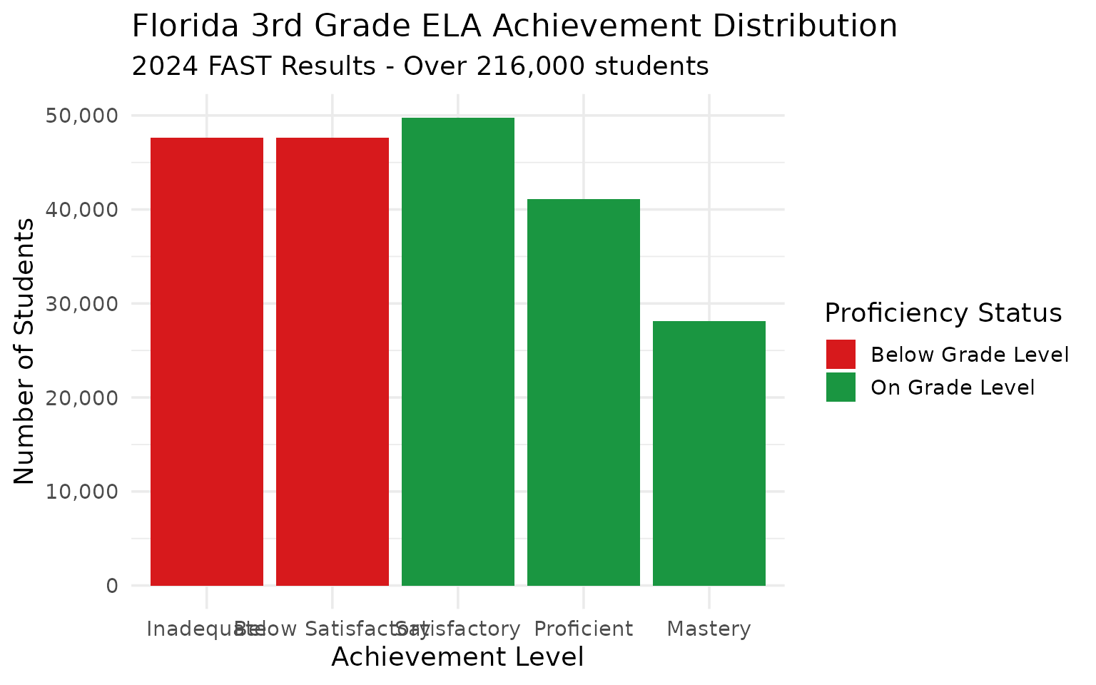
stopifnot(nrow(central) > 0)14. The tidy format enables trend analysis
Using tidy = TRUE makes it easy to analyze achievement
level distributions.
tidy_assess <- fetch_assessment(2024, "ela", grade = 3, level = "district",
                                 tidy = TRUE, use_cache = TRUE)

tidy_state <- tidy_assess |>
  filter(is_state) |>
  select(proficiency_level, proficiency_label, pct, n_students, is_proficient)

tidy_state
#> # A tibble: 5 × 5
#>   proficiency_level proficiency_label    pct n_students is_proficient
#>   <chr>             <chr>              <dbl>      <dbl> <lgl>
#> 1 level_1           Inadequate            22      47624 FALSE
#> 2 level_2           Below Satisfactory    22      47624 FALSE
#> 3 level_3           Satisfactory          23      49789 TRUE
#> 4 level_4           Proficient            19      41130 TRUE
#> 5 level_5           Mastery               13      28141 TRUE
stopifnot(nrow(tidy_state) > 0)
tidy_state |>
  mutate(proficiency_label = factor(proficiency_label,
    levels = c("Inadequate", "Below Satisfactory", "Satisfactory", "Proficient", "Mastery"))) |>
  ggplot(aes(x = proficiency_label, y = n_students, fill = is_proficient)) +
  geom_col() +
  scale_y_continuous(labels = scales::comma) +
  scale_fill_manual(values = c("FALSE" = "#D7191C", "TRUE" = "#1A9641"),
                    labels = c("Below Grade Level", "On Grade Level")) +
  labs(
    title = "Florida 3rd Grade ELA Achievement Distribution",
    subtitle = "2024 FAST Results - Over 216,000 students",
    x = "Achievement Level",
    y = "Number of Students",
    fill = "Proficiency Status"
  )
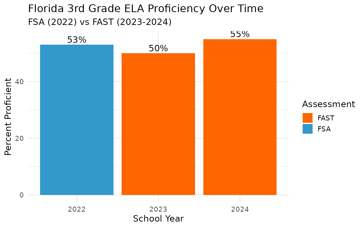
15. Multi-year data shows assessment transition effects
Comparing FSA (2022) to FAST (2023-2024) shows the impact of assessment changes.
multi_year <- tryCatch({
  fetch_assessment_multi(c(2022, 2023, 2024), "ela", grade = 3,
                         level = "district", tidy = FALSE, use_cache = TRUE) |>
    filter(is_state) |>
    select(end_year, assessment_system, n_tested, pct_proficient)
}, error = function(e) {
  warning("Some assessment years may not be available: ", conditionMessage(e))
  data.frame(end_year = integer(0), assessment_system = character(0),
             n_tested = integer(0), pct_proficient = numeric(0))
})

multi_year
#> # A tibble: 3 × 4
#>   end_year assessment_system n_tested pct_proficient
#>      <dbl> <chr>                <dbl>          <dbl>
#> 1     2022 FSA                 210287             53
#> 2     2023 FAST                221504             50
#> 3     2024 FAST                216473             55
stopifnot(nrow(multi_year) > 0)
multi_year |>
  ggplot(aes(x = factor(end_year), y = pct_proficient, fill = assessment_system)) +
  geom_col() +
  geom_text(aes(label = paste0(pct_proficient, "%")), vjust = -0.3) +
  scale_fill_manual(values = c("FSA" = "#3399CC", "FAST" = "#FF6600")) +
  labs(
    title = "Florida 3rd Grade ELA Proficiency Over Time",
    subtitle = "FSA (2022) vs FAST (2023-2024)",
    x = "School Year",
    y = "Percent Proficient",
    fill = "Assessment"
  )
Data Notes
Assessment Data Source: Florida Department of Education (FLDOE) https://www.fldoe.org/accountability/assessments/k-12-student-assessment/results/
Available Years: - 2019, 2022-2025 (no 2020/2021 due to COVID-19 testing waiver)
Subjects: - ELA Reading: Grades 3-10 - Mathematics: Grades 3-8
Suppression Rules: - Results may be suppressed for small n-sizes to protect student privacy
Summary
Florida’s assessment data reveals significant patterns:
- Scale: Over 216,000 3rd graders tested, making Florida one of the largest testing programs
- Proficiency: 55% of 3rd graders read on grade level (Level 3+)
- Equity gaps: 40+ percentage point gap between highest and lowest performing districts
- Regional patterns: Lab schools and affluent suburbs outperform rural Panhandle counties
- Intervention needs: 22% of 3rd graders at Level 1 need intensive support
- Grade trends: ELA proficiency rises with grade level; Math proficiency peaks early
These patterns inform policy decisions about literacy interventions, resource allocation, and accountability.
Data sourced from the Florida Department of Education.
sessionInfo()
#> R version 4.5.2 (2025-10-31)
#> Platform: x86_64-pc-linux-gnu
#> Running under: Ubuntu 24.04.3 LTS
#>
#> Matrix products: default
#> BLAS:   /usr/lib/x86_64-linux-gnu/openblas-pthread/libblas.so.3
#> LAPACK: /usr/lib/x86_64-linux-gnu/openblas-pthread/libopenblasp-r0.3.26.so;  LAPACK version 3.12.0
#>
#> locale:
#>  [1] LC_CTYPE=C.UTF-8       LC_NUMERIC=C           LC_TIME=C.UTF-8
#>  [4] LC_COLLATE=C.UTF-8     LC_MONETARY=C.UTF-8    LC_MESSAGES=C.UTF-8
#>  [7] LC_PAPER=C.UTF-8       LC_NAME=C              LC_ADDRESS=C
#> [10] LC_TELEPHONE=C         LC_MEASUREMENT=C.UTF-8 LC_IDENTIFICATION=C
#>
#> time zone: UTC
#> tzcode source: system (glibc)
#>
#> attached base packages:
#> [1] stats     graphics  grDevices utils     datasets  methods   base
#>
#> other attached packages:
#> [1] ggplot2_4.0.2      tidyr_1.3.2        dplyr_1.2.0        flschooldata_0.1.0
#>
#> loaded via a namespace (and not attached):
#>  [1] gtable_0.3.6       jsonlite_2.0.0     compiler_4.5.2     tidyselect_1.2.1
#>  [5] jquerylib_0.1.4    systemfonts_1.3.2  scales_1.4.0       textshaping_1.0.5
#>  [9] readxl_1.4.5       yaml_2.3.12        fastmap_1.2.0      R6_2.6.1
#> [13] labeling_0.4.3     generics_0.1.4     curl_7.0.0         knitr_1.51
#> [17] forcats_1.0.1      tibble_3.3.1       desc_1.4.3         bslib_0.10.0
#> [21] pillar_1.11.1      RColorBrewer_1.1-3 rlang_1.1.7        utf8_1.2.6
#> [25] cachem_1.1.0       xfun_0.56          S7_0.2.1           fs_1.6.7
#> [29] sass_0.4.10        cli_3.6.5          withr_3.0.2        pkgdown_2.2.0
#> [33] magrittr_2.0.4     digest_0.6.39      grid_4.5.2         rappdirs_0.3.4
#> [37] lifecycle_1.0.5    vctrs_0.7.1        evaluate_1.0.5     glue_1.8.0
#> [41] cellranger_1.1.0   farver_2.1.2       codetools_0.2-20   ragg_1.5.1
#> [45] httr_1.4.8         rmarkdown_2.30     purrr_1.2.1        tools_4.5.2
#> [49] pkgconfig_2.0.3    htmltools_0.5.9