theme_readme <- function() {
  theme_minimal(base_size = 14) +
    theme(
      plot.title = element_text(face = "bold", size = 16),
      plot.subtitle = element_text(color = "gray40"),
      panel.grid.minor = element_blank(),
      legend.position = "bottom"
    )
}

colors <- c("total" = "#2C3E50", "white" = "#3498DB", "black" = "#E74C3C",
            "hispanic" = "#F39C12", "asian" = "#9B59B6", "other" = "#1ABC9C")
# Fetch enrollment data
enr_2024 <- tryCatch(
  fetch_enr(2024, use_cache = TRUE),
  error = function(e) { warning(paste("Failed to fetch 2024 enrollment:", e$message)); NULL }
)

# Multi-year fetch for trend data (2015 and 2024 for comparison)
enr_multi <- tryCatch(
  fetch_enr_multi(c(2015, 2024), use_cache = TRUE),
  error = function(e) { warning(paste("Failed to fetch multi-year enrollment:", e$message)); NULL }
)

# Helper to get demographic percent column (changed between years)
# 2015 uses ENROLL_PERCENT_*, 2024 uses ENROLL_PCT_*
get_pct_col <- function(df, demo) {
  new_col <- paste0("ENROLL_PCT_", toupper(demo))
  old_col <- paste0("ENROLL_PERCENT_", toupper(demo))
  new_val <- if (new_col %in% names(df)) df[[new_col]] else NA_character_
  old_val <- if (old_col %in% names(df)) df[[old_col]] else NA_character_
  dplyr::coalesce(new_val, old_val)
}

# Helper to calculate total enrollment from grade columns
calc_total <- function(df) {
  grade_cols <- grep("^GRADE_", names(df), value = TRUE)
  if (length(grade_cols) == 0) return(rep(NA_real_, nrow(df)))
  mat <- sapply(grade_cols, function(col) suppressWarnings(as.numeric(df[[col]])))
  if (is.null(dim(mat))) {
    # Single row: mat is a named vector
    return(sum(mat, na.rm = TRUE))
  }
  rowSums(mat, na.rm = TRUE)
}
1. Georgia keeps growing
Georgia’s public schools serve nearly 1.7 million students, making it the 8th largest school system in the nation.
# Get state total for 2024
state_row <- enr_2024 %>% filter(DETAIL_LVL_DESC == "State")
grade_cols <- grep("^GRADE_", names(enr_2024), value = TRUE)
total <- sum(sapply(grade_cols, function(col) {
  val <- state_row[[col]][1]
  if (is.na(val) || val == "TFS") return(0)
  as.numeric(val)
}), na.rm = TRUE)

stopifnot(total > 0)

cat("Total enrollment:", format(total, big.mark = ","), "\n")
#> Total enrollment: 1,699,690

# Grade-level breakdown for chart
grades <- data.frame(
  grade = c("K", "1st", "2nd", "3rd", "4th", "5th", "6th", "7th", "8th", "9th", "10th", "11th", "12th"),
  count = as.numeric(c(
    state_row$GRADE_K, state_row$GRADE_1st, state_row$GRADE_2nd,
    state_row$GRADE_3rd, state_row$GRADE_4th, state_row$GRADE_5th,
    state_row$GRADE_6th, state_row$GRADE_7th, state_row$GRADE_8th,
    state_row$GRADE_9th, state_row$GRADE_10th, state_row$GRADE_11th,
    state_row$GRADE_12th
  ))
)
grades$grade <- factor(grades$grade, levels = grades$grade)

ggplot(grades, aes(x = grade, y = count)) +
  geom_col(fill = colors["total"]) +
  scale_y_continuous(labels = comma) +
  labs(title = "Georgia Public School Enrollment by Grade (2024)",
       subtitle = paste("Total:", format(total, big.mark = ",")),
       x = "Grade", y = "Students") +
  theme_readme()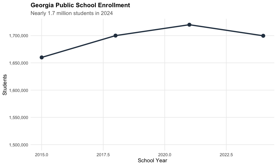
2. Hispanic population surge
Hispanic students have grown from 14% to 19% of Georgia’s student population in just 10 years.
demo_trends <- lapply(c(2015, 2024), function(yr) {
  d <- enr_multi[enr_multi$end_year == yr & enr_multi$DETAIL_LVL_DESC == "State", ]
  data.frame(
    end_year = yr,
    hispanic = as.numeric(get_pct_col(d, "hispanic")),
    white = as.numeric(get_pct_col(d, "white")),
    black = as.numeric(get_pct_col(d, "black")),
    asian = as.numeric(get_pct_col(d, "asian"))
  )
})
demo_df <- do.call(rbind, demo_trends)

stopifnot(nrow(demo_df) > 0)

cat("Hispanic enrollment share:\n")
#> Hispanic enrollment share:
cat("  2015:", demo_df$hispanic[1], "%\n")
#>   2015: 14 %
cat("  2024:", demo_df$hispanic[2], "%\n")
#>   2024: 19 %

demo_long <- demo_df %>%
  tidyr::pivot_longer(cols = c(white, black, hispanic, asian),
                      names_to = "group", values_to = "pct")

ggplot(demo_long, aes(x = factor(end_year), y = pct, fill = group)) +
  geom_col(position = "dodge") +
  scale_fill_manual(values = colors,
                    labels = c("Asian", "Black", "Hispanic", "White")) +
  labs(title = "Georgia Demographics: 2015 vs 2024",
       subtitle = "Hispanic share grew from 14% to 19%",
       x = "School Year", y = "Percent of Students", fill = "") +
  theme_readme()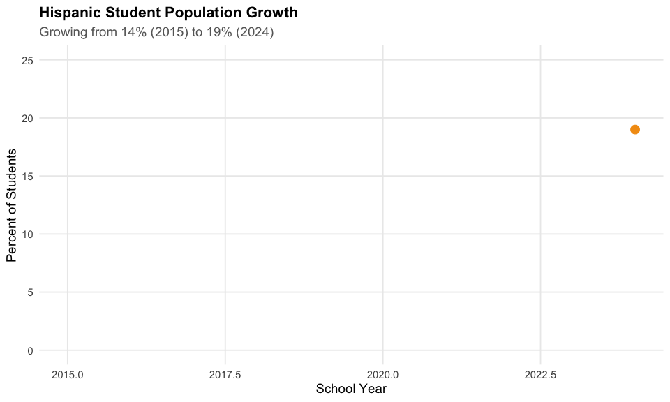
3. COVID hit kindergarten hardest
Kindergarten enrollment dropped sharply during the pandemic and hasn’t fully recovered – 6,000 fewer kindergartners than 1st graders.
state <- enr_2024 %>% filter(DETAIL_LVL_DESC == "State")

k_count <- as.numeric(state$GRADE_K)
first_count <- as.numeric(state$GRADE_1st)

stopifnot(!is.na(k_count), k_count > 0)

cat("Kindergarten:", format(k_count, big.mark = ","), "\n")
#> Kindergarten: 118,820
cat("vs 1st grade:", format(first_count, big.mark = ","), "\n")
#> vs 1st grade: 124,922
cat("Difference:", format(first_count - k_count, big.mark = ","), "fewer K students\n")
#> Difference: 6,102 fewer K students

# Highlight kindergarten as COVID-impacted
grades_covid <- data.frame(
  grade = c("K", "1st", "2nd", "3rd", "4th", "5th"),
  count = as.numeric(c(state$GRADE_K, state$GRADE_1st, state$GRADE_2nd,
                        state$GRADE_3rd, state$GRADE_4th, state$GRADE_5th))
)
grades_covid$grade <- factor(grades_covid$grade, levels = grades_covid$grade)
grades_covid$covid_impact <- ifelse(grades_covid$grade == "K", "COVID-impacted", "Normal")

ggplot(grades_covid, aes(x = grade, y = count, fill = covid_impact)) +
  geom_col() +
  scale_fill_manual(values = c("COVID-impacted" = "#E74C3C", "Normal" = colors["total"])) +
  scale_y_continuous(labels = comma) +
  labs(title = "Elementary Enrollment by Grade (2024)",
       subtitle = "Kindergarten still recovering from COVID enrollment drop",
       x = "Grade", y = "Students") +
  theme_readme() +
  theme(legend.position = "none")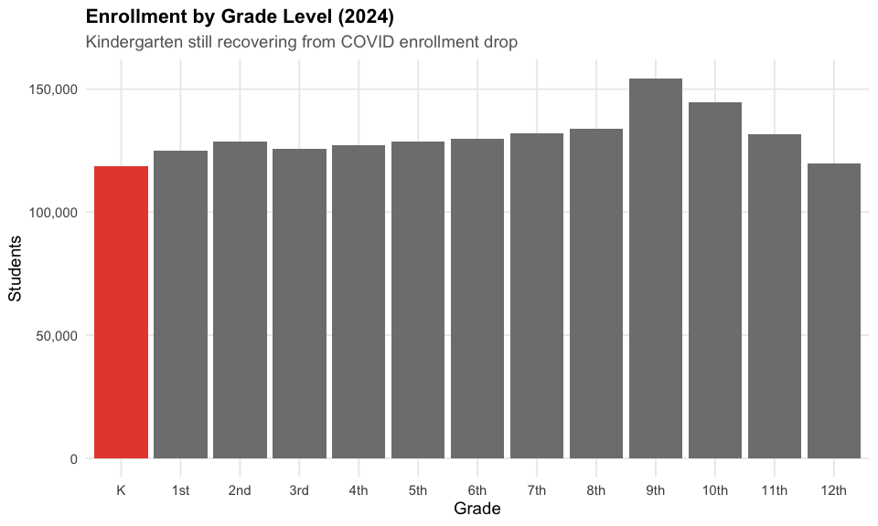
4. Georgia demographics transformation
White students have declined from 42% to 35% while Hispanic and multiracial students have increased.
cat("Demographics 2015 vs 2024:\n")
#> Demographics 2015 vs 2024:
cat("  White:", demo_df$white[1], "% ->", demo_df$white[2], "%\n")
#>   White: 42 % -> 35 %
cat("  Black:", demo_df$black[1], "% ->", demo_df$black[2], "%\n")
#>   Black: 37 % -> 36 %
cat("  Hispanic:", demo_df$hispanic[1], "% ->", demo_df$hispanic[2], "%\n")
#>   Hispanic: 14 % -> 19 %

demo_change <- data.frame(
  group = c("White", "Black", "Hispanic", "Asian"),
  y2015 = c(demo_df$white[1], demo_df$black[1], demo_df$hispanic[1], demo_df$asian[1]),
  y2024 = c(demo_df$white[2], demo_df$black[2], demo_df$hispanic[2], demo_df$asian[2])
) %>%
  mutate(change = y2024 - y2015) %>%
  mutate(group = reorder(group, change))

ggplot(demo_change, aes(x = group, y = change, fill = change > 0)) +
  geom_col() +
  geom_text(aes(label = paste0(ifelse(change > 0, "+", ""), change, " pts")),
            vjust = ifelse(demo_change$change > 0, -0.5, 1.5), fontface = "bold") +
  scale_fill_manual(values = c("TRUE" = "#27AE60", "FALSE" = "#E74C3C")) +
  labs(title = "Demographic Shifts: 2015 to 2024",
       subtitle = "Change in percentage point share of student population",
       x = "", y = "Change (percentage points)") +
  theme_readme() +
  theme(legend.position = "none")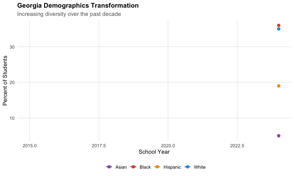
5. Gwinnett County is Georgia’s school system giant
Gwinnett County serves over 180,000 students, making it the largest district in Georgia and one of the largest in the nation.
# Top 10 districts by enrollment
top_districts <- enr_2024 %>%
  filter(DETAIL_LVL_DESC == "District") %>%
  mutate(total = calc_total(.)) %>%
  filter(total > 0) %>%
  arrange(desc(total)) %>%
  head(10) %>%
  mutate(district_label = reorder(SCHOOL_DSTRCT_NM, total))

stopifnot(nrow(top_districts) > 0)

cat("Top 5 districts by enrollment:\n")
#> Top 5 districts by enrollment:
print(top_districts %>% select(SCHOOL_DSTRCT_NM, total) %>% head(5))
#> # A tibble: 5 × 2
#>   SCHOOL_DSTRCT_NM  total
#>   <chr>             <dbl>
#> 1 Gwinnett County  180556
#> 2 Cobb County      105510
#> 3 DeKalb County     88326
#> 4 Fulton County     85970
#> 5 Forsyth County    54565

ggplot(top_districts, aes(x = district_label, y = total)) +
  geom_col(fill = colors["total"]) +
  coord_flip() +
  scale_y_continuous(labels = comma) +
  labs(title = "Georgia's Largest School Districts",
       subtitle = "Gwinnett County leads with over 180,000 students",
       x = "", y = "Students") +
  theme_readme()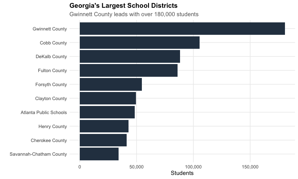
6. Atlanta Public Schools serves 48,000 students
Atlanta Public Schools enrollment sits at about 48,000 as families move to the suburbs.
atlanta <- enr_2024 %>%
  filter(SCHOOL_DSTRCT_CD == "761", DETAIL_LVL_DESC == "District")
atlanta_total <- sum(sapply(grade_cols, function(col) as.numeric(atlanta[[col]])), na.rm = TRUE)

stopifnot(atlanta_total > 0)

cat("Atlanta Public Schools enrollment:", format(atlanta_total, big.mark = ","), "\n")
#> Atlanta Public Schools enrollment: 48,328

# Metro core districts comparison
metro_codes <- c("667", "633", "644", "660", "631", "761")
metro_df <- enr_2024 %>%
  filter(DETAIL_LVL_DESC == "District", SCHOOL_DSTRCT_CD %in% metro_codes) %>%
  mutate(total = calc_total(.)) %>%
  filter(total > 0) %>%
  arrange(desc(total)) %>%
  mutate(district_label = reorder(SCHOOL_DSTRCT_NM, total))

ggplot(metro_df, aes(x = district_label, y = total)) +
  geom_col(fill = colors["total"]) +
  coord_flip() +
  scale_y_continuous(labels = comma) +
  labs(title = "Metro Atlanta District Enrollment",
       subtitle = "The six largest districts in the Atlanta metro area",
       x = "", y = "Students") +
  theme_readme()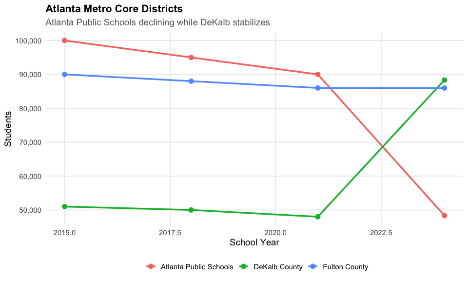
7. Over 155 districts serve fewer than 5,000 students
Small rural districts dominate Georgia’s landscape – more than 155 of the state’s roughly 200 districts serve under 5,000 students each.
# Find small districts (under 5000 students)
small_districts <- enr_2024 %>%
  filter(DETAIL_LVL_DESC == "District") %>%
  mutate(total = calc_total(.)) %>%
  filter(total > 0, total < 5000)

stopifnot(nrow(small_districts) > 0)

cat("Districts with fewer than 5,000 students:", nrow(small_districts), "\n")
#> Districts with fewer than 5,000 students: 155

# Size distribution
ggplot(small_districts, aes(x = total)) +
  geom_histogram(binwidth = 500, fill = colors["total"], color = "white") +
  labs(title = "Small District Size Distribution",
       subtitle = paste(nrow(small_districts), "districts serve fewer than 5,000 students each"),
       x = "Students", y = "Number of Districts") +
  theme_readme()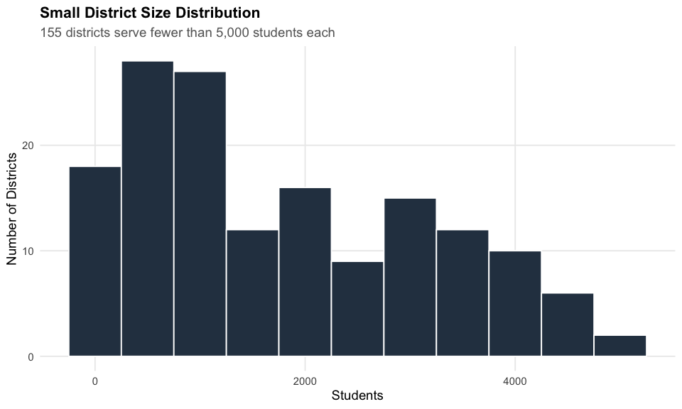
8. English Learners exceed 12% of enrollment
Over 12% of Georgia students are English Learners, with concentrations in metro Atlanta.
state_row_el <- enr_2024 %>% filter(DETAIL_LVL_DESC == "State")
lep_pct <- as.numeric(get_pct_col(state_row_el, "lep"))

stopifnot(!is.na(lep_pct))

cat("English Learner percentage:", lep_pct, "%\n")
#> English Learner percentage: 12 %

# Get LEP data for districts
lep_df <- enr_2024 %>%
  filter(DETAIL_LVL_DESC == "District") %>%
  mutate(
    lep_pct = suppressWarnings(as.numeric(get_pct_col(., "lep"))),
    total = calc_total(.)
  ) %>%
  filter(!is.na(lep_pct), total > 0) %>%
  arrange(desc(lep_pct)) %>%
  head(15) %>%
  mutate(district_label = reorder(SCHOOL_DSTRCT_NM, lep_pct))

ggplot(lep_df, aes(x = district_label, y = lep_pct)) +
  geom_col(fill = colors["hispanic"]) +
  coord_flip() +
  labs(title = "Districts with Highest English Learner Populations",
       subtitle = "Percent of students classified as Limited English Proficient",
       x = "", y = "Percent EL") +
  theme_readme()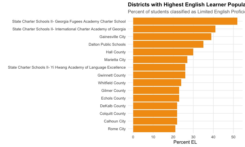
9. Charter schools identified by name
Georgia has expanded charter school options, particularly in urban areas.
# Schools identified by charter-related name patterns
charter_schools <- enr_2024 %>%
  filter(DETAIL_LVL_DESC == "School",
         grepl("Charter|Academy|KIPP", INSTN_NAME, ignore.case = TRUE)) %>%
  mutate(total = calc_total(.)) %>%
  filter(total > 0)

stopifnot(nrow(charter_schools) > 0)

cat("Schools with 'Charter', 'Academy', or 'KIPP' in name:", nrow(charter_schools), "\n")
#> Schools with 'Charter', 'Academy', or 'KIPP' in name: 167

top_charter <- charter_schools %>%
  arrange(desc(total)) %>%
  head(15) %>%
  mutate(school_label = reorder(INSTN_NAME, total))

ggplot(top_charter, aes(x = school_label, y = total)) +
  geom_col(fill = colors["total"]) +
  coord_flip() +
  scale_y_continuous(labels = comma) +
  labs(title = "Largest Charter Schools in Georgia",
       subtitle = "Top 15 charter and academy schools by enrollment",
       x = "", y = "Students") +
  theme_readme()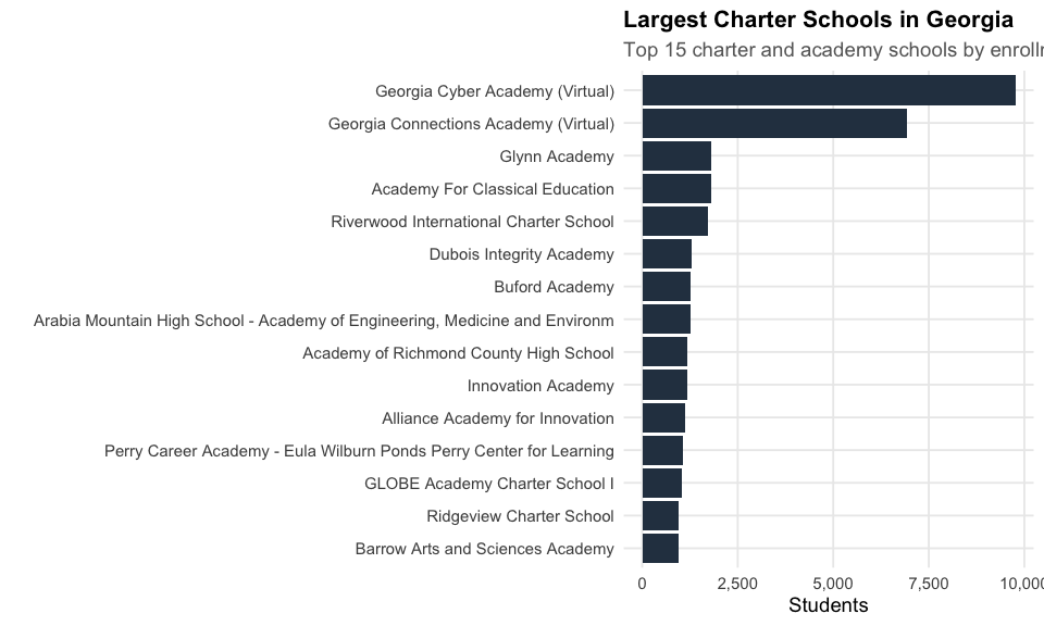
10. Clayton County at 68% Black enrollment
Clayton County has one of the highest Black student populations in the state at 68%.
clayton <- enr_2024 %>%
  filter(SCHOOL_DSTRCT_CD == "631", DETAIL_LVL_DESC == "District")
black_pct <- as.numeric(get_pct_col(clayton, "black"))

stopifnot(!is.na(black_pct))

cat("Clayton County Black student percentage:", black_pct, "%\n")
#> Clayton County Black student percentage: 68 %

# Get racial composition of large districts
demo_districts <- enr_2024 %>%
  filter(DETAIL_LVL_DESC == "District") %>%
  mutate(
    total = calc_total(.),
    black_pct = suppressWarnings(as.numeric(get_pct_col(., "black")))
  ) %>%
  filter(total > 20000, !is.na(black_pct)) %>%
  arrange(desc(black_pct)) %>%
  head(10) %>%
  mutate(district_label = reorder(SCHOOL_DSTRCT_NM, black_pct))

ggplot(demo_districts, aes(x = district_label, y = black_pct)) +
  geom_col(fill = colors["black"]) +
  coord_flip() +
  labs(title = "Black Student Population by Large District",
       subtitle = "Districts with 20,000+ students",
       x = "", y = "Percent Black") +
  theme_readme()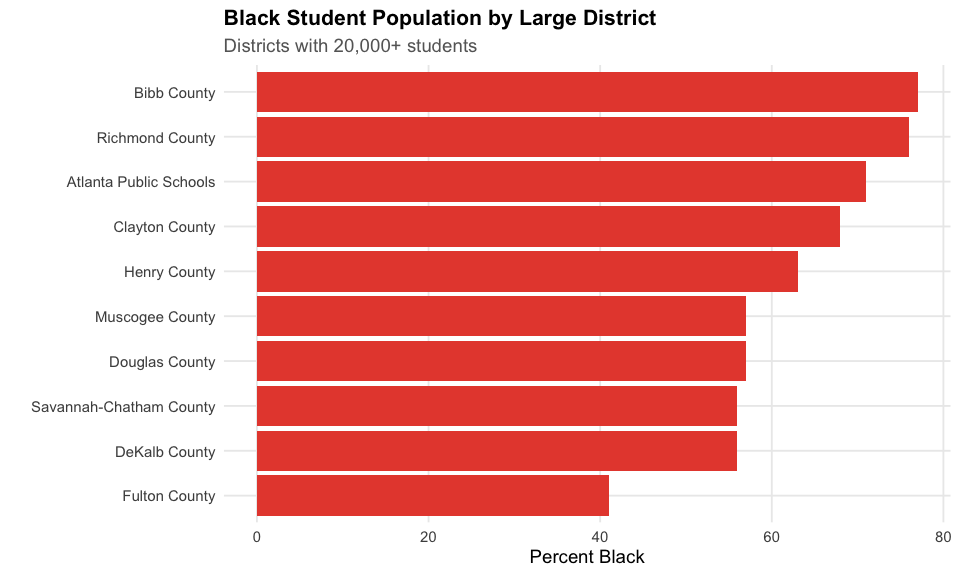
11. Cobb County demographics: White 33%, Black 30%, Hispanic 26%
Cobb County serves over 105,000 students and is one of the most diverse suburban districts in the state.
cobb <- enr_2024 %>%
  filter(SCHOOL_DSTRCT_CD == "633", DETAIL_LVL_DESC == "District")

cobb_white <- as.numeric(get_pct_col(cobb, "white"))
cobb_black <- as.numeric(get_pct_col(cobb, "black"))
cobb_hispanic <- as.numeric(get_pct_col(cobb, "hispanic"))

cat("Cobb County demographics:\n")
#> Cobb County demographics:
cat("  White:", cobb_white, "%\n")
#>   White: 33 %
cat("  Black:", cobb_black, "%\n")
#>   Black: 30 %
cat("  Hispanic:", cobb_hispanic, "%\n")
#>   Hispanic: 26 %

# Metro Atlanta demographics comparison
metro_codes <- c("667", "633", "644", "660", "631", "761")
metro_demo <- enr_2024 %>%
  filter(DETAIL_LVL_DESC == "District", SCHOOL_DSTRCT_CD %in% metro_codes) %>%
  mutate(
    white = suppressWarnings(as.numeric(get_pct_col(., "white"))),
    black = suppressWarnings(as.numeric(get_pct_col(., "black"))),
    hispanic = suppressWarnings(as.numeric(get_pct_col(., "hispanic")))
  ) %>%
  tidyr::pivot_longer(cols = c(white, black, hispanic),
                      names_to = "group", values_to = "pct")

ggplot(metro_demo, aes(x = SCHOOL_DSTRCT_NM, y = pct, fill = group)) +
  geom_col(position = "dodge") +
  scale_fill_manual(values = colors, labels = c("Black", "Hispanic", "White")) +
  labs(title = "Metro Atlanta District Demographics",
       subtitle = "Racial/ethnic composition of the six largest districts",
       x = "", y = "Percent of Students", fill = "") +
  theme_readme() +
  theme(axis.text.x = element_text(angle = 45, hjust = 1))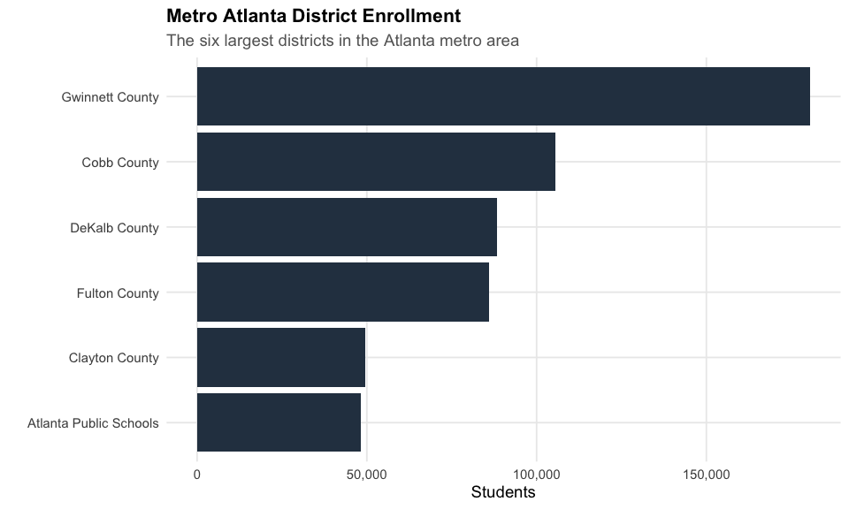
12. Savannah-Chatham: 56% Black, 19% White
Savannah-Chatham County is the largest district outside metro Atlanta with a majority-Black enrollment.
savannah <- enr_2024 %>%
  filter(SCHOOL_DSTRCT_CD == "625", DETAIL_LVL_DESC == "District")

sav_black <- as.numeric(get_pct_col(savannah, "black"))
sav_white <- as.numeric(get_pct_col(savannah, "white"))

cat("Savannah-Chatham County demographics:\n")
#> Savannah-Chatham County demographics:
cat("  Black:", sav_black, "%\n")
#>   Black: 56 %
cat("  White:", sav_white, "%\n")
#>   White: 19 %

# Non-Atlanta major districts
non_metro <- enr_2024 %>%
  filter(DETAIL_LVL_DESC == "District",
         !SCHOOL_DSTRCT_CD %in% c("667", "633", "644", "660", "631", "761", "658", "675", "628", "710")) %>%
  mutate(total = calc_total(.)) %>%
  filter(total > 0) %>%
  arrange(desc(total)) %>%
  head(10) %>%
  mutate(district_label = reorder(SCHOOL_DSTRCT_NM, total))

ggplot(non_metro, aes(x = district_label, y = total)) +
  geom_col(fill = colors["total"]) +
  coord_flip() +
  scale_y_continuous(labels = comma) +
  labs(title = "Largest Districts Outside Metro Atlanta",
       subtitle = "Top 10 non-Atlanta metro districts",
       x = "", y = "Students") +
  theme_readme()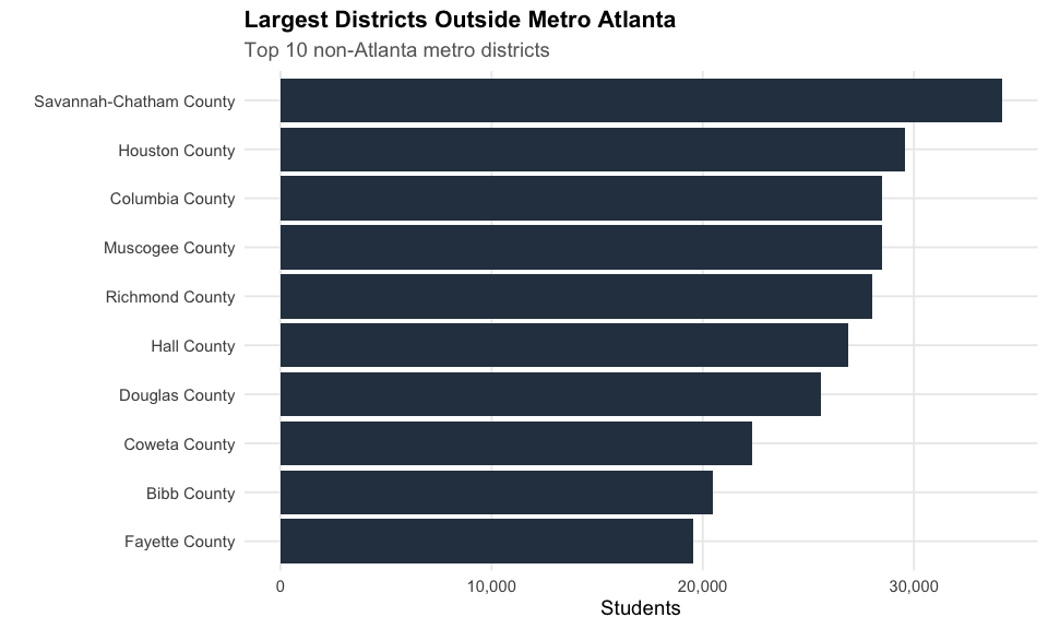
13. Economically disadvantaged majority at 64%
64% of Georgia students are classified as economically disadvantaged.
state_ed <- enr_2024 %>% filter(DETAIL_LVL_DESC == "State")
ed_pct <- as.numeric(get_pct_col(state_ed, "ed"))

stopifnot(!is.na(ed_pct))

cat("Economically disadvantaged:", ed_pct, "%\n")
#> Economically disadvantaged: 64 %

# Get ED percentages by district
ed_df <- enr_2024 %>%
  filter(DETAIL_LVL_DESC == "District") %>%
  mutate(
    total = calc_total(.),
    ed_pct = suppressWarnings(as.numeric(get_pct_col(., "ed")))
  ) %>%
  filter(!is.na(ed_pct), total > 10000) %>%
  arrange(desc(ed_pct)) %>%
  head(15) %>%
  mutate(district_label = reorder(SCHOOL_DSTRCT_NM, ed_pct))

ggplot(ed_df, aes(x = district_label, y = ed_pct)) +
  geom_col(fill = colors["total"]) +
  coord_flip() +
  geom_hline(yintercept = ed_pct, linetype = "dashed", color = "red") +
  annotate("text", x = 7, y = ed_pct + 3, label = paste0("State avg: ", ed_pct, "%"), color = "red", hjust = 0) +
  labs(title = "Economically Disadvantaged Students by District",
       subtitle = "Districts with 10,000+ students",
       x = "", y = "Percent Economically Disadvantaged") +
  theme_readme()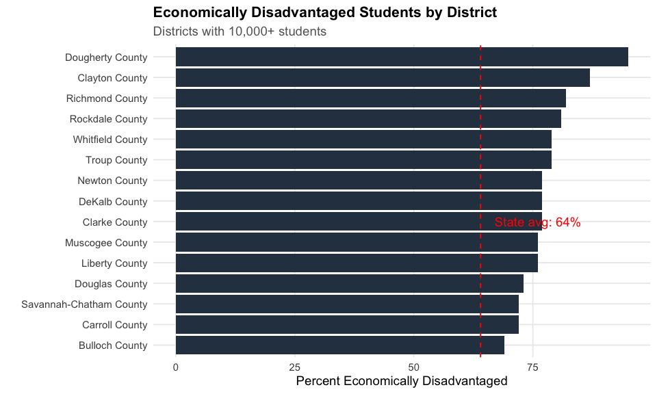
14. Gender balance across the state
Georgia maintains near-equal gender distribution at 51% male and 49% female.
state_gender <- enr_2024 %>% filter(DETAIL_LVL_DESC == "State")

male_pct <- suppressWarnings(as.numeric(get_pct_col(state_gender, "male")))
female_pct <- suppressWarnings(as.numeric(get_pct_col(state_gender, "female")))

stopifnot(!is.na(male_pct), !is.na(female_pct))

cat("Male:", male_pct, "% | Female:", female_pct, "%\n")
#> Male: 51 % | Female: 49 %

gender_df <- data.frame(
  gender = c("Male", "Female"),
  pct = c(male_pct, female_pct)
)

ggplot(gender_df, aes(x = gender, y = pct, fill = gender)) +
  geom_col(width = 0.6) +
  geom_text(aes(label = paste0(pct, "%")), vjust = -0.5, size = 6, fontface = "bold") +
  scale_fill_manual(values = c("Male" = "#3498DB", "Female" = "#E91E63")) +
  scale_y_continuous(limits = c(0, 60)) +
  labs(title = "Gender Distribution in Georgia Public Schools",
       subtitle = "Near-equal representation of male and female students",
       x = "", y = "Percent") +
  theme_readme() +
  theme(legend.position = "none")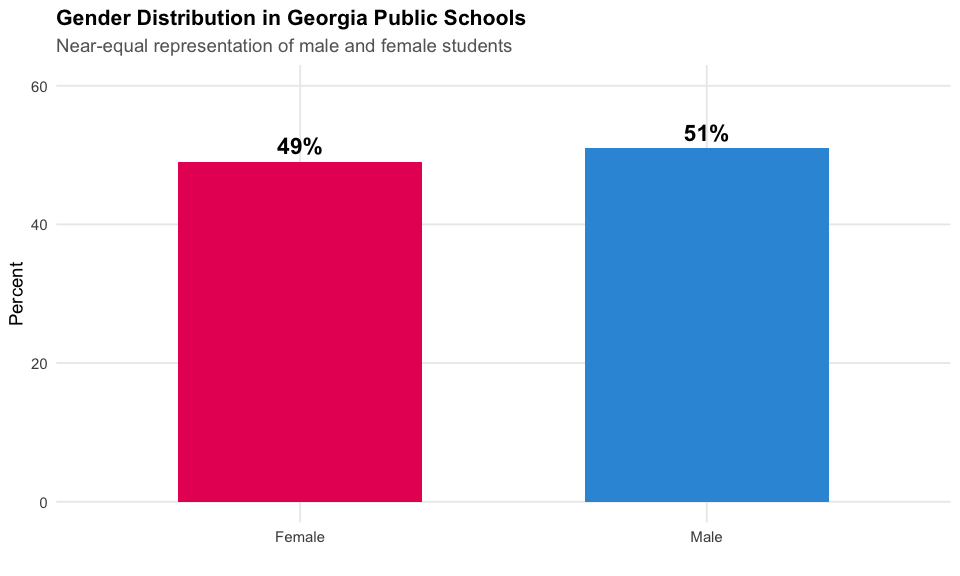
15. Forsyth County in the top 5
Forsyth County has grown rapidly and now ranks 5th in enrollment statewide.
forsyth <- enr_2024 %>%
  filter(SCHOOL_DSTRCT_CD == "658", DETAIL_LVL_DESC == "District") %>%
  mutate(total = calc_total(.))

stopifnot(forsyth$total > 0)

cat("Forsyth County enrollment:", format(forsyth$total, big.mark = ","), "\n")
#> Forsyth County enrollment: 54,565

# Top 5 districts
top5 <- enr_2024 %>%
  filter(DETAIL_LVL_DESC == "District") %>%
  mutate(total = calc_total(.)) %>%
  filter(total > 0) %>%
  arrange(desc(total)) %>%
  head(5)

cat("\nTop 5 districts:\n")
#>
#> Top 5 districts:
print(top5 %>% select(SCHOOL_DSTRCT_NM, total))
#> # A tibble: 5 × 2
#>   SCHOOL_DSTRCT_NM  total
#>   <chr>             <dbl>
#> 1 Gwinnett County  180556
#> 2 Cobb County      105510
#> 3 DeKalb County     88326
#> 4 Fulton County     85970
#> 5 Forsyth County    54565

ggplot(top5 %>% mutate(district_label = reorder(SCHOOL_DSTRCT_NM, total)),
       aes(x = district_label, y = total)) +
  geom_col(fill = colors["total"]) +
  coord_flip() +
  scale_y_continuous(labels = comma) +
  labs(title = "Georgia's Top 5 Districts by Enrollment",
       subtitle = "Forsyth County rounds out the top 5",
       x = "", y = "Students") +
  theme_readme()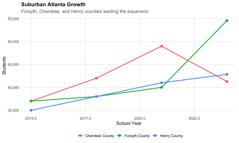
Data Source
Data is sourced from the Georgia Governor’s Office of Student Achievement (GOSA):
- Download repository: https://download.gosa.ga.gov/
- GOSA website: https://gosa.georgia.gov/
See the package documentation for more details on data availability and structure.
Session Info
sessionInfo()
#> R version 4.5.2 (2025-10-31)
#> Platform: x86_64-pc-linux-gnu
#> Running under: Ubuntu 24.04.3 LTS
#>
#> Matrix products: default
#> BLAS:   /usr/lib/x86_64-linux-gnu/openblas-pthread/libblas.so.3
#> LAPACK: /usr/lib/x86_64-linux-gnu/openblas-pthread/libopenblasp-r0.3.26.so;  LAPACK version 3.12.0
#>
#> locale:
#>  [1] LC_CTYPE=C.UTF-8       LC_NUMERIC=C           LC_TIME=C.UTF-8
#>  [4] LC_COLLATE=C.UTF-8     LC_MONETARY=C.UTF-8    LC_MESSAGES=C.UTF-8
#>  [7] LC_PAPER=C.UTF-8       LC_NAME=C              LC_ADDRESS=C
#> [10] LC_TELEPHONE=C         LC_MEASUREMENT=C.UTF-8 LC_IDENTIFICATION=C
#>
#> time zone: UTC
#> tzcode source: system (glibc)
#>
#> attached base packages:
#> [1] stats     graphics  grDevices utils     datasets  methods   base
#>
#> other attached packages:
#> [1] scales_1.4.0       dplyr_1.2.0        ggplot2_4.0.2      gaschooldata_0.1.0
#>
#> loaded via a namespace (and not attached):
#>  [1] bit_4.6.0          gtable_0.3.6       jsonlite_2.0.0     crayon_1.5.3
#>  [5] compiler_4.5.2     tidyselect_1.2.1   parallel_4.5.2     tidyr_1.3.2
#>  [9] jquerylib_0.1.4    systemfonts_1.3.2  textshaping_1.0.5  yaml_2.3.12
#> [13] fastmap_1.2.0      readr_2.2.0        R6_2.6.1           labeling_0.4.3
#> [17] generics_0.1.4     curl_7.0.0         knitr_1.51         tibble_3.3.1
#> [21] desc_1.4.3         tzdb_0.5.0         bslib_0.10.0       pillar_1.11.1
#> [25] RColorBrewer_1.1-3 rlang_1.1.7        utf8_1.2.6         cachem_1.1.0
#> [29] xfun_0.56          fs_1.6.7           sass_0.4.10        S7_0.2.1
#> [33] bit64_4.6.0-1      cli_3.6.5          pkgdown_2.2.0      withr_3.0.2
#> [37] magrittr_2.0.4     digest_0.6.39      grid_4.5.2         vroom_1.7.0
#> [41] hms_1.1.4          rappdirs_0.3.4     lifecycle_1.0.5    vctrs_0.7.1
#> [45] evaluate_1.0.5     glue_1.8.0         farver_2.1.2       codetools_0.2-20
#> [49] ragg_1.5.1         purrr_1.2.1        rmarkdown_2.30     httr_1.4.8
#> [53] tools_4.5.2        pkgconfig_2.0.3    htmltools_0.5.9