Georgia Milestones Assessment Trends
Source:vignettes/georgia-assessment.Rmd
georgia-assessment.Rmd
theme_readme <- function() {
  theme_minimal(base_size = 14) +
    theme(
      plot.title = element_text(face = "bold", size = 16),
      plot.subtitle = element_text(color = "gray40"),
      panel.grid.minor = element_blank(),
      legend.position = "bottom"
    )
}

colors <- c(
  "proficient" = "#27AE60", "distinguished" = "#2ECC71",
  "developing" = "#F39C12", "beginning" = "#E74C3C",
  "total" = "#2C3E50", "ela" = "#3498DB", "math" = "#9B59B6",
  "science" = "#1ABC9C", "social_studies" = "#E67E22"
)
# Fetch 2024 assessment data (both EOG and EOC)
assess_2024 <- tryCatch(
  fetch_assessment(2024, use_cache = TRUE),
  error = function(e) { warning(paste("Failed to fetch assessment data:", e$message)); NULL }
)

# Also get EOG only for cleaner grade-level analysis
eog_2024 <- tryCatch(
  fetch_eog(2024, use_cache = TRUE),
  error = function(e) { warning(paste("Failed to fetch EOG data:", e$message)); NULL }
)
eoc_2024 <- tryCatch(
  fetch_eoc(2024, use_cache = TRUE),
  error = function(e) { warning(paste("Failed to fetch EOC data:", e$message)); NULL }
)

# Wide format for some analyses
assess_wide <- tryCatch(
  fetch_assessment(2024, tidy = FALSE, use_cache = TRUE),
  error = function(e) { warning(paste("Failed to fetch wide assessment data:", e$message)); NULL }
)
1. Fewer than half of Georgia students are proficient in ELA
Statewide proficiency remains a challenge, with fewer than half of students meeting grade-level standards in English Language Arts.
# State-level proficiency for All Students, ELA, All Grades
# Filter to state aggregate row (district_id == "ALL", school_id == "ALL")
ela_state <- assess_wide %>%
  filter(district_id == "ALL", school_id == "ALL",
         subgroup == "All Students",
         subject == "ELA",
         grade == "All") %>%
  filter(!is.na(n_tested))

stopifnot(nrow(ela_state) > 0)

ela_state <- ela_state %>%
  mutate(
    n_prof_dist = n_proficient + n_distinguished,
    pct_proficient = n_prof_dist / n_tested * 100
  )

cat("State ELA Proficiency (All Students):\n")
#> State ELA Proficiency (All Students):
cat("  Students tested:", format(ela_state$n_tested, big.mark = ","), "\n")
#>   Students tested: 759,126
cat("  Percent proficient or distinguished:", round(ela_state$pct_proficient, 1), "%\n")
#>   Percent proficient or distinguished: 41.8 %
# Proficiency breakdown for ELA (state-level from tidy EOG)
ela_prof <- eog_2024 %>%
  filter(district_id == "ALL", school_id == "ALL",
         subgroup == "All Students", subject == "ELA", grade == "All") %>%
  group_by(proficiency_level) %>%
  summarize(n = sum(n_students, na.rm = TRUE), .groups = "drop") %>%
  mutate(pct = n / sum(n) * 100,
         proficiency_level = factor(proficiency_level,
                                     levels = c("beginning", "developing", "proficient", "distinguished")))

stopifnot(nrow(ela_prof) > 0)

ggplot(ela_prof, aes(x = proficiency_level, y = pct, fill = proficiency_level)) +
  geom_col() +
  geom_text(aes(label = paste0(round(pct, 1), "%")), vjust = -0.5, fontface = "bold") +
  scale_fill_manual(values = c("beginning" = colors["beginning"],
                               "developing" = colors["developing"],
                               "proficient" = colors["proficient"],
                               "distinguished" = colors["distinguished"])) +
  scale_y_continuous(limits = c(0, 50)) +
  labs(title = "Georgia Milestones ELA Proficiency (2024)",
       subtitle = "All Students, All Grades Combined",
       x = "Proficiency Level", y = "Percent of Students") +
  theme_readme() +
  theme(legend.position = "none")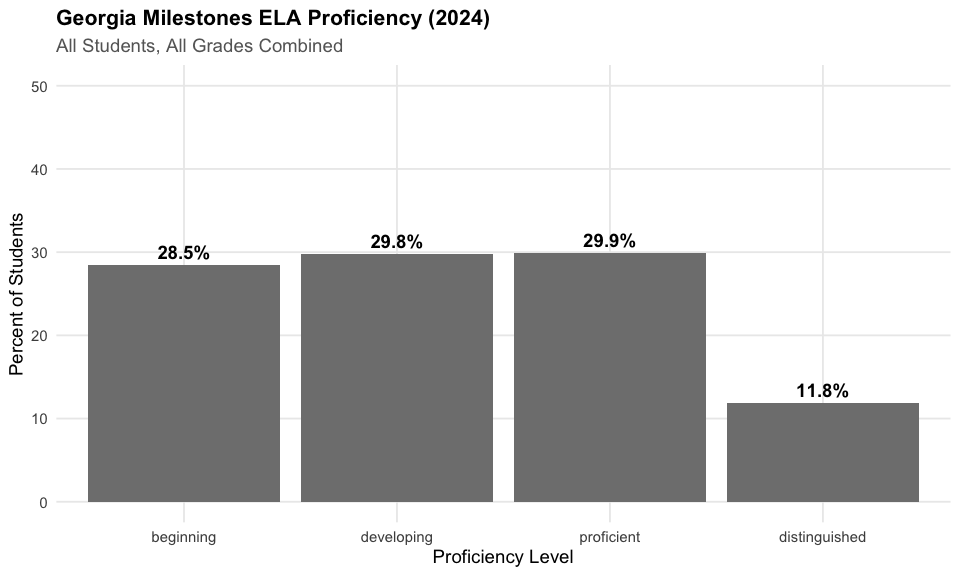
2. Math and ELA proficiency are nearly identical at 42%
Math and ELA both land around 42% proficiency statewide, with fewer than half of students meeting grade-level standards.
math_state <- assess_wide %>%
  filter(district_id == "ALL", school_id == "ALL",
         subgroup == "All Students",
         subject == "Math",
         grade == "All") %>%
  filter(!is.na(n_tested))

stopifnot(nrow(math_state) > 0)

math_state <- math_state %>%
  mutate(
    n_prof_dist = n_proficient + n_distinguished,
    pct_proficient = n_prof_dist / n_tested * 100
  )

cat("State Math Proficiency (All Students):\n")
#> State Math Proficiency (All Students):
cat("  Students tested:", format(math_state$n_tested, big.mark = ","), "\n")
#>   Students tested: 758,385
cat("  Percent proficient or distinguished:", round(math_state$pct_proficient, 1), "%\n")
#>   Percent proficient or distinguished: 41.8 %
math_prof <- eog_2024 %>%
  filter(district_id == "ALL", school_id == "ALL",
         subgroup == "All Students", subject == "Math", grade == "All") %>%
  group_by(proficiency_level) %>%
  summarize(n = sum(n_students, na.rm = TRUE), .groups = "drop") %>%
  mutate(pct = n / sum(n) * 100,
         proficiency_level = factor(proficiency_level,
                                     levels = c("beginning", "developing", "proficient", "distinguished")))

stopifnot(nrow(math_prof) > 0)

ggplot(math_prof, aes(x = proficiency_level, y = pct, fill = proficiency_level)) +
  geom_col() +
  geom_text(aes(label = paste0(round(pct, 1), "%")), vjust = -0.5, fontface = "bold") +
  scale_fill_manual(values = c("beginning" = colors["beginning"],
                               "developing" = colors["developing"],
                               "proficient" = colors["proficient"],
                               "distinguished" = colors["distinguished"])) +
  scale_y_continuous(limits = c(0, 50)) +
  labs(title = "Georgia Milestones Math Proficiency (2024)",
       subtitle = "All Students, All Grades Combined",
       x = "Proficiency Level", y = "Percent of Students") +
  theme_readme() +
  theme(legend.position = "none")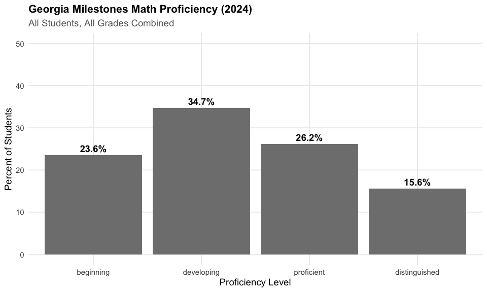
3. Economically disadvantaged students face a 10-point proficiency gap
The achievement gap between economically disadvantaged students and all students is about 10 percentage points in ELA.
econ_compare <- assess_wide %>%
  filter(district_id == "ALL", school_id == "ALL",
         subgroup %in% c("All Students", "Economically Disadvantaged"),
         subject == "ELA",
         grade == "All") %>%
  filter(!is.na(n_tested)) %>%
  mutate(
    n_prof_dist = n_proficient + n_distinguished,
    pct_proficient = n_prof_dist / n_tested * 100
  ) %>%
  select(subgroup, n_tested, n_prof_dist, pct_proficient)

stopifnot(nrow(econ_compare) == 2)

cat("ELA Proficiency Gap:\n")
#> ELA Proficiency Gap:
print(econ_compare)
#>                     subgroup n_tested n_prof_dist pct_proficient
#> 1               All Students   759126      317242       41.79043
#> 2 Economically Disadvantaged   535542      169218       31.59752
cat("\nGap:", round(abs(diff(econ_compare$pct_proficient)), 1), "percentage points\n")
#>
#> Gap: 10.2 percentage points
subgroup_gaps <- assess_wide %>%
  filter(district_id == "ALL", school_id == "ALL",
         subgroup %in% c("All Students", "Economically Disadvantaged",
                         "Students with Disabilities", "English Learners"),
         subject == "ELA",
         grade == "All") %>%
  filter(!is.na(n_tested)) %>%
  mutate(pct_proficient = (n_proficient + n_distinguished) / n_tested * 100) %>%
  select(subgroup, pct_proficient) %>%
  mutate(subgroup = reorder(subgroup, pct_proficient))

stopifnot(nrow(subgroup_gaps) > 0)

ggplot(subgroup_gaps, aes(x = subgroup, y = pct_proficient, fill = subgroup)) +
  geom_col() +
  geom_text(aes(label = paste0(round(pct_proficient, 1), "%")), hjust = -0.1, fontface = "bold") +
  coord_flip() +
  scale_y_continuous(limits = c(0, 60)) +
  labs(title = "ELA Proficiency by Student Subgroup",
       subtitle = "Significant gaps persist for economically disadvantaged and SWD students",
       x = "", y = "Percent Proficient") +
  theme_readme() +
  theme(legend.position = "none")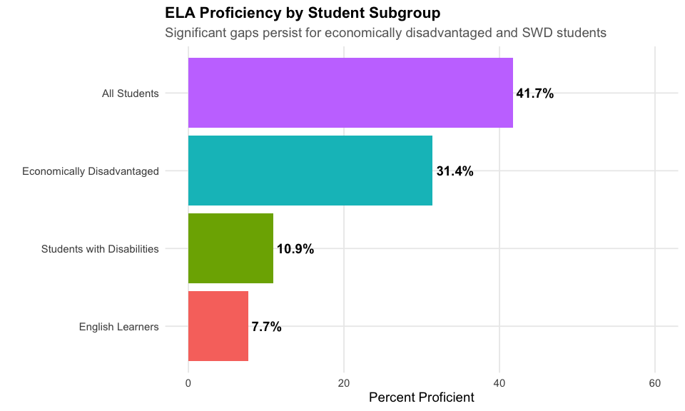
4. Asian students lead at 72% ELA proficiency
Racial achievement gaps remain substantial in Georgia, with Asian students at 72% proficiency and Black students at 29%.
race_gaps <- assess_wide %>%
  filter(district_id == "ALL", school_id == "ALL",
         subgroup %in% c("All Students", "White", "Black", "Hispanic", "Asian"),
         subject == "ELA",
         grade == "All") %>%
  filter(!is.na(n_tested)) %>%
  mutate(pct_proficient = (n_proficient + n_distinguished) / n_tested * 100)

stopifnot(nrow(race_gaps) > 0)

cat("ELA Proficiency by Race/Ethnicity:\n")
#> ELA Proficiency by Race/Ethnicity:
print(race_gaps %>% arrange(desc(pct_proficient)) %>% select(subgroup, n_tested, pct_proficient))
#>       subgroup n_tested pct_proficient
#> 1        Asian    40321       72.19563
#> 2        White   261411       55.03556
#> 3 All Students   759126       41.79043
#> 4     Hispanic   147351       31.21933
#> 5        Black   270916       29.34895
race_gaps_sorted <- race_gaps %>%
  filter(subgroup != "All Students") %>%
  mutate(subgroup = reorder(subgroup, pct_proficient))

ggplot(race_gaps_sorted, aes(x = subgroup, y = pct_proficient, fill = subgroup)) +
  geom_col() +
  geom_text(aes(label = paste0(round(pct_proficient, 1), "%")), hjust = -0.1, fontface = "bold") +
  coord_flip() +
  scale_y_continuous(limits = c(0, 85)) +
  labs(title = "ELA Proficiency by Race/Ethnicity",
       subtitle = "Asian students lead while Black students face largest gap",
       x = "", y = "Percent Proficient") +
  theme_readme() +
  theme(legend.position = "none")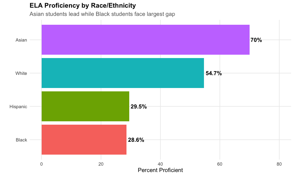
5. Asian students dominate across all subjects
Asian students achieve 72% in ELA, 79% in Math, and 69% in Science – far ahead of every other group.
asian_subjects <- assess_wide %>%
  filter(district_id == "ALL", school_id == "ALL",
         subgroup == "Asian",
         subject %in% c("ELA", "Math", "Science"),
         grade == "All") %>%
  filter(!is.na(n_tested)) %>%
  mutate(pct_proficient = (n_proficient + n_distinguished) / n_tested * 100)

stopifnot(nrow(asian_subjects) > 0)

cat("Asian Student Proficiency by Subject:\n")
#> Asian Student Proficiency by Subject:
print(asian_subjects %>% select(subject, n_tested, pct_proficient))
#>   subject n_tested pct_proficient
#> 1     ELA    40321       72.19563
#> 2    Math    40302       79.14992
#> 3 Science     8856       68.91373
ggplot(asian_subjects, aes(x = subject, y = pct_proficient)) +
  geom_col(fill = colors["math"]) +
  geom_text(aes(label = paste0(round(pct_proficient, 1), "%")), vjust = -0.5, fontface = "bold") +
  scale_y_continuous(limits = c(0, 90)) +
  labs(title = "Asian Student Proficiency by Subject",
       subtitle = "Consistently high performance across all tested subjects",
       x = "Subject", y = "Percent Proficient") +
  theme_readme()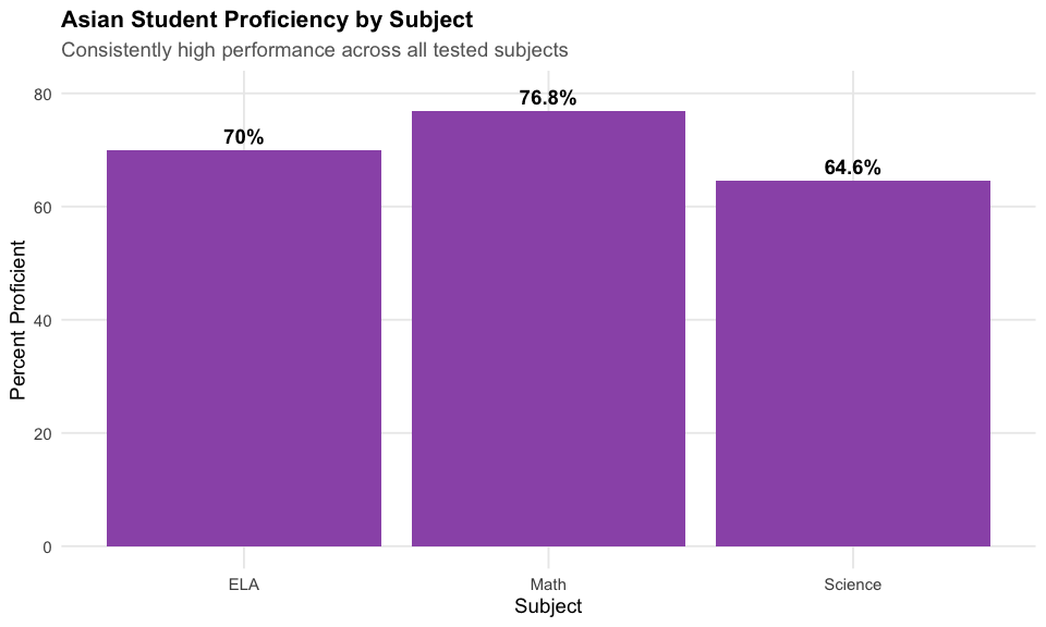
6. Girls outperform boys in ELA by 9 points
Gender gaps persist in literacy, with girls at 46% proficient vs boys at 38%.
gender_ela <- assess_wide %>%
  filter(district_id == "ALL", school_id == "ALL",
         subgroup %in% c("Male", "Female"),
         subject == "ELA",
         grade == "All") %>%
  filter(!is.na(n_tested)) %>%
  mutate(pct_proficient = (n_proficient + n_distinguished) / n_tested * 100)

stopifnot(nrow(gender_ela) == 2)

gender_math <- assess_wide %>%
  filter(district_id == "ALL", school_id == "ALL",
         subgroup %in% c("Male", "Female"),
         subject == "Math",
         grade == "All") %>%
  filter(!is.na(n_tested)) %>%
  mutate(pct_proficient = (n_proficient + n_distinguished) / n_tested * 100)

stopifnot(nrow(gender_math) == 2)

cat("Gender Gaps in ELA:\n")
#> Gender Gaps in ELA:
print(gender_ela %>% select(subgroup, n_tested, pct_proficient))
#>   subgroup n_tested pct_proficient
#> 1     Male   385928       37.45025
#> 2   Female   373198       46.27865
cat("\nGender Gaps in Math:\n")
#>
#> Gender Gaps in Math:
print(gender_math %>% select(subgroup, n_tested, pct_proficient))
#>   subgroup n_tested pct_proficient
#> 1     Male   385518       43.57073
#> 2   Female   372867       40.01105
gender_all <- bind_rows(
  gender_ela %>% mutate(subject = "ELA"),
  gender_math %>% mutate(subject = "Math")
)

ggplot(gender_all, aes(x = subject, y = pct_proficient, fill = subgroup)) +
  geom_col(position = "dodge") +
  geom_text(aes(label = paste0(round(pct_proficient, 1), "%")),
            position = position_dodge(0.9), vjust = -0.5, fontface = "bold") +
  scale_fill_manual(values = c("Female" = "#E91E63", "Male" = "#2196F3")) +
  scale_y_continuous(limits = c(0, 60)) +
  labs(title = "Proficiency by Gender",
       subtitle = "Girls outperform in ELA; near-parity in Math",
       x = "Subject", y = "Percent Proficient", fill = "") +
  theme_readme()
7. Gwinnett County tests over 81,000 students
Gwinnett County is the largest testing district in Georgia by far, with nearly double the next-largest district.
district_counts <- assess_wide %>%
  filter(school_id == "ALL", district_id != "ALL",
         subgroup == "All Students",
         subject == "ELA",
         grade == "All") %>%
  filter(!is.na(n_tested)) %>%
  arrange(desc(n_tested)) %>%
  head(10) %>%
  mutate(district_label = reorder(district_name, n_tested))

stopifnot(nrow(district_counts) > 0)

cat("Largest Districts by Students Tested (ELA):\n")
#> Largest Districts by Students Tested (ELA):
print(district_counts %>% select(district_name, n_tested))
#>              district_name n_tested
#> 1          Gwinnett County    81271
#> 2              Cobb County    46257
#> 3            DeKalb County    39731
#> 4            Fulton County    37069
#> 5           Forsyth County    25229
#> 6   Atlanta Public Schools    22325
#> 7           Clayton County    22110
#> 8             Henry County    18462
#> 9          Cherokee County    18399
#> 10 Savannah-Chatham County    15508
ggplot(district_counts, aes(x = district_label, y = n_tested)) +
  geom_col(fill = colors["total"]) +
  coord_flip() +
  scale_y_continuous(labels = comma) +
  labs(title = "Largest Districts by Assessment Volume",
       subtitle = "Students tested in ELA (All Grades)",
       x = "", y = "Students Tested") +
  theme_readme()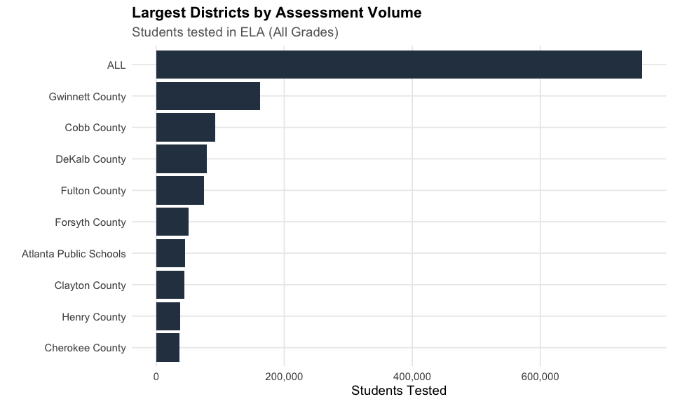
8. Decatur City leads with 74% ELA proficiency
The highest-performing districts in Georgia reach 60-74% proficiency, far above the 42% state average.
district_proficiency <- assess_wide %>%
  filter(school_id == "ALL", district_id != "ALL",
         subgroup == "All Students",
         subject == "ELA",
         grade == "All") %>%
  filter(!is.na(n_tested)) %>%
  mutate(pct_proficient = (n_proficient + n_distinguished) / n_tested * 100) %>%
  filter(n_tested >= 1000) %>%
  arrange(desc(pct_proficient)) %>%
  head(15) %>%
  mutate(district_label = reorder(district_name, pct_proficient))

stopifnot(nrow(district_proficiency) > 0)

cat("Highest-Performing Districts (ELA, 1000+ students):\n")
#> Highest-Performing Districts (ELA, 1000+ students):
print(district_proficiency %>% select(district_name, pct_proficient, n_tested) %>% head(10))
#>              district_name pct_proficient n_tested
#> 1  City Schools of Decatur       74.41305     2513
#> 2            Oconee County       72.11690     3798
#> 3              Bremen City       67.50000     1000
#> 4           Fayette County       65.77706     8693
#> 5              Buford City       65.56586     2695
#> 6           Jefferson City       64.75495     1918
#> 7           Forsyth County       62.06746    25229
#> 8          Columbia County       58.79690    13033
#> 9             Bryan County       57.37634     4650
#> 10           Pierce County       55.28507     1561
ggplot(district_proficiency, aes(x = district_label, y = pct_proficient)) +
  geom_col(fill = colors["proficient"]) +
  coord_flip() +
  geom_hline(yintercept = 42, linetype = "dashed", color = "red") +
  annotate("text", x = 5, y = 45, label = "State avg: 42%", color = "red", hjust = 0) +
  labs(title = "Highest-Performing Districts in ELA",
       subtitle = "Districts with 1,000+ students tested",
       x = "", y = "Percent Proficient") +
  theme_readme()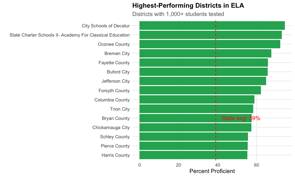
9. US History has the lowest EOC proficiency at 39%
End-of-Course exams show US History as the most challenging high school subject, while Biology leads at 45%.
eoc_wide <- tryCatch(
  fetch_eoc(2024, tidy = FALSE, use_cache = TRUE),
  error = function(e) { warning(paste("Failed to fetch EOC wide data:", e$message)); NULL }
)

eoc_prof_wide <- eoc_wide %>%
  filter(district_id == "ALL", school_id == "ALL",
         subgroup == "All Students", grade == "All") %>%
  filter(!is.na(n_tested)) %>%
  mutate(pct_proficient = (n_proficient + n_distinguished) / n_tested * 100) %>%
  filter(!is.na(pct_proficient), n_tested > 10000) %>%
  arrange(pct_proficient) %>%
  mutate(subject = reorder(subject, pct_proficient))

stopifnot(nrow(eoc_prof_wide) > 0)

cat("EOC Subject Proficiency:\n")
#> EOC Subject Proficiency:
print(eoc_prof_wide %>% select(subject, n_tested, pct_proficient))
#>               subject n_tested pct_proficient
#> 1          US History   100363       38.83104
#> 2 American Lit & Comp   132797       41.97158
#> 3   Algebra: Concepts   145998       44.11704
#> 4             Biology   139223       44.84532
ggplot(eoc_prof_wide, aes(x = subject, y = pct_proficient)) +
  geom_col(fill = colors["total"]) +
  coord_flip() +
  geom_text(aes(label = paste0(round(pct_proficient, 1), "%")), hjust = -0.1, fontface = "bold") +
  scale_y_continuous(limits = c(0, 55)) +
  labs(title = "End-of-Course Exam Proficiency by Subject",
       subtitle = "High school subject proficiency rates for 2024",
       x = "", y = "Percent Proficient") +
  theme_readme()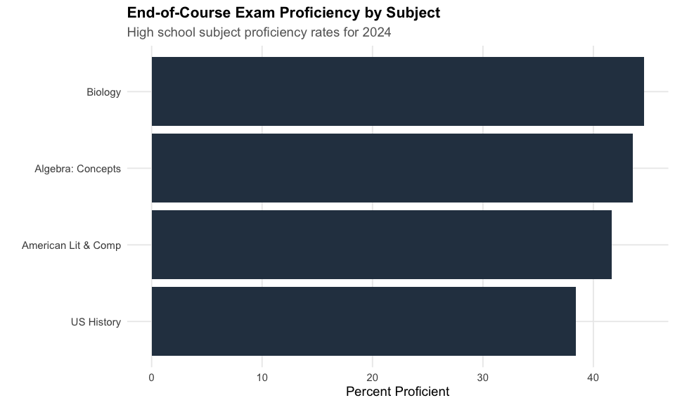
10. American Literature proficiency sits at 42%
The American Literature EOC shows that high school literacy remains a challenge with 42% proficiency.
am_lit <- eoc_wide %>%
  filter(district_id == "ALL", school_id == "ALL",
         subject == "American Lit & Comp",
         subgroup == "All Students",
         grade == "All") %>%
  filter(!is.na(n_tested)) %>%
  mutate(pct_proficient = (n_proficient + n_distinguished) / n_tested * 100)

stopifnot(nrow(am_lit) > 0)

cat("American Literature and Composition Proficiency:\n")
#> American Literature and Composition Proficiency:
cat("  Students tested:", format(am_lit$n_tested, big.mark = ","), "\n")
#>   Students tested: 132,797
cat("  Percent proficient:", round(am_lit$pct_proficient, 1), "%\n")
#>   Percent proficient: 42 %
eoc_ela <- eoc_2024 %>%
  filter(district_id == "ALL", school_id == "ALL",
         subject == "American Lit & Comp",
         subgroup == "All Students",
         grade == "All") %>%
  group_by(subject, proficiency_level) %>%
  summarize(n = sum(n_students, na.rm = TRUE), .groups = "drop") %>%
  group_by(subject) %>%
  mutate(pct = n / sum(n) * 100) %>%
  mutate(proficiency_level = factor(proficiency_level,
                                     levels = c("beginning", "developing", "proficient", "distinguished")))

stopifnot(nrow(eoc_ela) > 0)

ggplot(eoc_ela, aes(x = proficiency_level, y = pct, fill = proficiency_level)) +
  geom_col() +
  geom_text(aes(label = paste0(round(pct, 1), "%")), vjust = -0.5, fontface = "bold") +
  scale_fill_manual(values = c("beginning" = colors["beginning"],
                               "developing" = colors["developing"],
                               "proficient" = colors["proficient"],
                               "distinguished" = colors["distinguished"])) +
  labs(title = "American Literature EOC Proficiency Breakdown",
       subtitle = "Proficiency level distribution for 2024",
       x = "Proficiency Level", y = "Percent of Students") +
  theme_readme() +
  theme(legend.position = "none")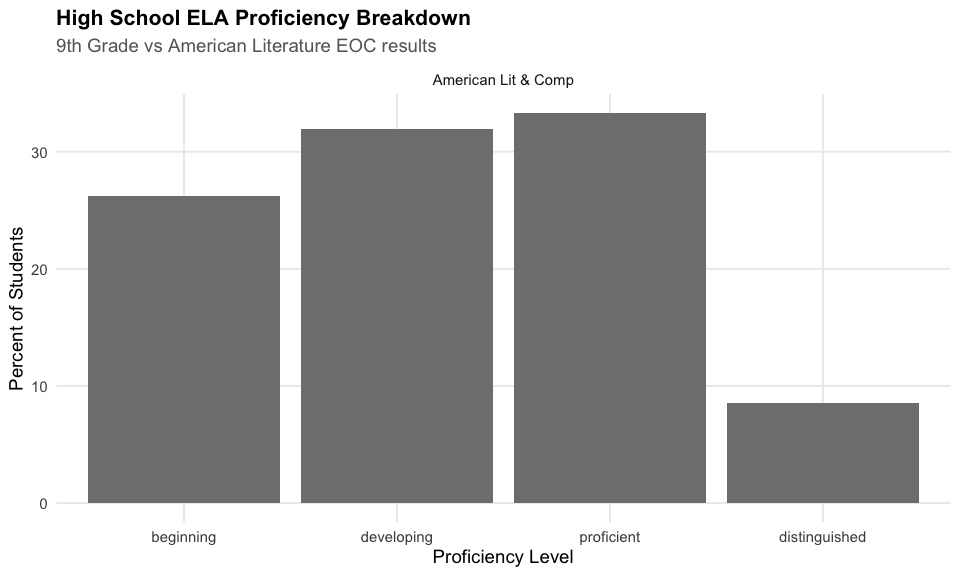
11. Students with Disabilities at 13% ELA proficiency
Students with Disabilities have the lowest proficiency rates across all subgroups, at 13% in ELA and 16% in Math.
swd_all <- assess_wide %>%
  filter(district_id == "ALL", school_id == "ALL",
         subgroup == "Students with Disabilities",
         subject %in% c("ELA", "Math"),
         grade == "All") %>%
  filter(!is.na(n_tested)) %>%
  mutate(pct_proficient = (n_proficient + n_distinguished) / n_tested * 100)

stopifnot(nrow(swd_all) > 0)

cat("Students with Disabilities Proficiency:\n")
#> Students with Disabilities Proficiency:
print(swd_all %>% select(subject, n_tested, pct_proficient))
#>   subject n_tested pct_proficient
#> 1     ELA   103604       13.21378
#> 2    Math   103447       16.47704
swd_compare <- assess_wide %>%
  filter(district_id == "ALL", school_id == "ALL",
         subgroup %in% c("All Students", "Students with Disabilities"),
         subject == "ELA",
         grade == "All") %>%
  filter(!is.na(n_tested)) %>%
  mutate(pct_proficient = (n_proficient + n_distinguished) / n_tested * 100)

stopifnot(nrow(swd_compare) > 0)

ggplot(swd_compare, aes(x = subgroup, y = pct_proficient, fill = subgroup)) +
  geom_col() +
  geom_text(aes(label = paste0(round(pct_proficient, 1), "%")), vjust = -0.5, fontface = "bold") +
  scale_fill_manual(values = c("All Students" = colors["total"],
                                "Students with Disabilities" = colors["beginning"])) +
  scale_y_continuous(limits = c(0, 55)) +
  labs(title = "ELA Proficiency: All Students vs Students with Disabilities",
       subtitle = "SWD students face a nearly 30-point gap",
       x = "", y = "Percent Proficient") +
  theme_readme() +
  theme(legend.position = "none")
12. English Learners face a 32-point ELA gap
English Learners achieve just 10% proficiency in ELA, compared to 42% statewide – a 32-point gap.
el_compare <- assess_wide %>%
  filter(district_id == "ALL", school_id == "ALL",
         subgroup %in% c("All Students", "English Learners"),
         subject %in% c("ELA", "Math"),
         grade == "All") %>%
  filter(!is.na(n_tested)) %>%
  mutate(pct_proficient = (n_proficient + n_distinguished) / n_tested * 100)

stopifnot(nrow(el_compare) > 0)

cat("English Learners vs All Students:\n")
#> English Learners vs All Students:
print(el_compare %>% select(subgroup, subject, n_tested, pct_proficient))
#>           subgroup subject n_tested pct_proficient
#> 1     All Students     ELA   759126      41.790427
#> 2     All Students    Math   758385      41.820579
#> 3 English Learners     ELA    75974       9.578277
#> 4 English Learners    Math    75906      17.470292
ggplot(el_compare, aes(x = subject, y = pct_proficient, fill = subgroup)) +
  geom_col(position = "dodge") +
  geom_text(aes(label = paste0(round(pct_proficient, 1), "%")),
            position = position_dodge(0.9), vjust = -0.5, fontface = "bold") +
  scale_fill_manual(values = c("All Students" = colors["total"],
                               "English Learners" = colors["developing"])) +
  scale_y_continuous(limits = c(0, 55)) +
  labs(title = "Proficiency: English Learners vs All Students",
       subtitle = "EL students face challenges in both ELA and Math",
       x = "Subject", y = "Percent Proficient", fill = "") +
  theme_readme()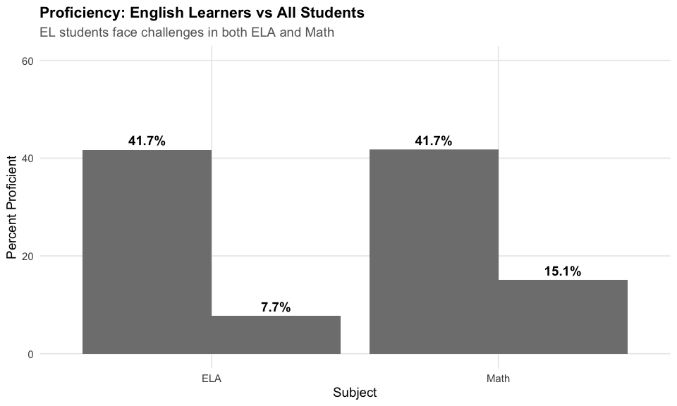
13. Only 12% reach Distinguished level in ELA
Just 12% of Georgia students achieve the highest proficiency level (Distinguished) in ELA.
# Use wide data for precise state-level distinguished count
dist_wide <- assess_wide %>%
  filter(district_id == "ALL", school_id == "ALL",
         subgroup == "All Students", subject == "ELA", grade == "All") %>%
  filter(!is.na(n_tested))

stopifnot(nrow(dist_wide) > 0)

pct_distinguished <- round(dist_wide$n_distinguished / dist_wide$n_tested * 100, 1)

cat("Distinguished Learners in ELA:\n")
#> Distinguished Learners in ELA:
cat("  Students tested:", format(dist_wide$n_tested, big.mark = ","), "\n")
#>   Students tested: 759,126
cat("  Distinguished count:", format(dist_wide$n_distinguished, big.mark = ","), "\n")
#>   Distinguished count: 90,270
cat("  Percent achieving Distinguished level:", pct_distinguished, "%\n")
#>   Percent achieving Distinguished level: 11.9 %
# Show proficiency level distribution for state-level ELA
prof_dist <- eog_2024 %>%
  filter(district_id == "ALL", school_id == "ALL",
         subgroup == "All Students", subject == "ELA", grade == "All") %>%
  mutate(proficiency_level = factor(proficiency_level,
                                     levels = c("beginning", "developing", "proficient", "distinguished")))

stopifnot(nrow(prof_dist) > 0)

ggplot(prof_dist, aes(x = proficiency_level, y = pct * 100, fill = proficiency_level)) +
  geom_col() +
  geom_text(aes(label = paste0(round(pct * 100, 1), "%")), vjust = -0.5, fontface = "bold") +
  scale_fill_manual(values = c("beginning" = colors["beginning"],
                               "developing" = colors["developing"],
                               "proficient" = colors["proficient"],
                               "distinguished" = colors["distinguished"])) +
  scale_y_continuous(limits = c(0, 50)) +
  labs(title = "ELA Proficiency Level Distribution (2024)",
       subtitle = "Only 12% of students reach the Distinguished level",
       x = "Proficiency Level", y = "Percent of Students") +
  theme_readme() +
  theme(legend.position = "none")
Data Notes
Data Source
Georgia Milestones assessment data from the Governor’s Office of Student Achievement (GOSA):
- Download repository: https://download.gosa.ga.gov/
- GOSA website: https://gosa.georgia.gov/
Assessment System
Georgia Milestones began in spring 2015, replacing the CRCT (Criterion-Referenced Competency Tests). The assessment includes:
- EOG (End of Grade): Grades 3-8 in ELA, Math; Science in grades 5 and 8; Social Studies in grade 8
- EOC (End of Course): High school courses including Algebra, Biology, US History, and American Literature
Proficiency Levels
- Beginning Learner: Does not yet demonstrate proficiency
- Developing Learner: Demonstrates partial proficiency
- Proficient Learner: Demonstrates proficiency in grade-level content
- Distinguished Learner: Demonstrates advanced proficiency
Session Info
sessionInfo()
#> R version 4.5.2 (2025-10-31)
#> Platform: x86_64-pc-linux-gnu
#> Running under: Ubuntu 24.04.3 LTS
#>
#> Matrix products: default
#> BLAS:   /usr/lib/x86_64-linux-gnu/openblas-pthread/libblas.so.3
#> LAPACK: /usr/lib/x86_64-linux-gnu/openblas-pthread/libopenblasp-r0.3.26.so;  LAPACK version 3.12.0
#>
#> locale:
#>  [1] LC_CTYPE=C.UTF-8       LC_NUMERIC=C           LC_TIME=C.UTF-8
#>  [4] LC_COLLATE=C.UTF-8     LC_MONETARY=C.UTF-8    LC_MESSAGES=C.UTF-8
#>  [7] LC_PAPER=C.UTF-8       LC_NAME=C              LC_ADDRESS=C
#> [10] LC_TELEPHONE=C         LC_MEASUREMENT=C.UTF-8 LC_IDENTIFICATION=C
#>
#> time zone: UTC
#> tzcode source: system (glibc)
#>
#> attached base packages:
#> [1] stats     graphics  grDevices utils     datasets  methods   base
#>
#> other attached packages:
#> [1] scales_1.4.0       dplyr_1.2.0        ggplot2_4.0.2      gaschooldata_0.1.0
#>
#> loaded via a namespace (and not attached):
#>  [1] bit_4.6.0          gtable_0.3.6       jsonlite_2.0.0     crayon_1.5.3
#>  [5] compiler_4.5.2     tidyselect_1.2.1   parallel_4.5.2     jquerylib_0.1.4
#>  [9] systemfonts_1.3.2  textshaping_1.0.5  yaml_2.3.12        fastmap_1.2.0
#> [13] readr_2.2.0        R6_2.6.1           labeling_0.4.3     generics_0.1.4
#> [17] curl_7.0.0         knitr_1.51         tibble_3.3.1       desc_1.4.3
#> [21] tzdb_0.5.0         bslib_0.10.0       pillar_1.11.1      RColorBrewer_1.1-3
#> [25] rlang_1.1.7        cachem_1.1.0       xfun_0.56          fs_1.6.7
#> [29] sass_0.4.10        S7_0.2.1           bit64_4.6.0-1      cli_3.6.5
#> [33] pkgdown_2.2.0      withr_3.0.2        magrittr_2.0.4     digest_0.6.39
#> [37] grid_4.5.2         vroom_1.7.0        hms_1.1.4          rappdirs_0.3.4
#> [41] lifecycle_1.0.5    vctrs_0.7.1        evaluate_1.0.5     glue_1.8.0
#> [45] farver_2.1.2       codetools_0.2-20   ragg_1.5.1         purrr_1.2.1
#> [49] rmarkdown_2.30     httr_1.4.8         tools_4.5.2        pkgconfig_2.0.3
#> [53] htmltools_0.5.9