Advanced-Coursework Access & Equity
Source:vignettes/nj-advanced-courses.Rmd
nj-advanced-courses.RmdThe usual AP/IB question is “how many students took an exam.” The
harder, more newsworthy question is about access: does
a school even offer advanced courses, and once offered, who actually
gets in. fetch_advanced_course_access() answers both. A
single front door over three NJ School Performance Report sheet
families:
-
type = "courses_offered"– one row per school per advanced course (enrolled / tested), 2017-2025. -
type = "participation_by_group"– AP/IB and dual-enrollment participation rates broken out by student group, 2021-2025. -
type = "sle"– Structured Learning Experience participation, 2017-2025.
Every rate and count comes straight from the published SPR workbooks;
suppression and no-data text is kept as NA, never a guessed
number.
The AP/IB access gap by student group
type = "participation_by_group" reports, for each
student group, the percent of students enrolled in one or more AP/IB
courses. The statewide rate per group is carried in the
apib_pct_state column. Lining the groups up shows an access
gap that is anything but subtle: in 2023-24 Asian students participated
at 70% while students with disabilities sat at
under 5%, with English learners, Black, Hispanic, and
economically disadvantaged students all well below the statewide
average.
groups <- c(
  "asian, native hawaiian, or pacific islander", "white", "multiracial",
  "total population", "hispanic", "black", "economically disadvantaged",
  "limited english proficiency", "students with disabilities"
)

apib_state <- fetch_advanced_course_access(
  2024, type = "participation_by_group", level = "district"
) %>%
  filter(is_state, subgroup %in% groups) %>%
  group_by(subgroup) %>%
  summarise(apib_pct = first(apib_pct_state), .groups = "drop") %>%
  filter(!is.na(apib_pct)) %>%
  arrange(apib_pct)

# Print-before-plot: confirm the data feeding the chart.
stopifnot(nrow(apib_state) > 0)
apib_state
#> # A tibble: 9 × 2
#>   subgroup                                    apib_pct
#>   <chr>                                          <dbl>
#> 1 students with disabilities                       4.8
#> 2 limited english proficiency                      9.8
#> 3 black                                           20.3
#> 4 economically disadvantaged                      22.8
#> 5 hispanic                                        23.2
#> 6 total population                                35.9
#> 7 multiracial                                     41
#> 8 white                                           41.8
#> 9 asian, native hawaiian, or pacific islander     70.5
ggplot(apib_state, aes(x = reorder(subgroup, apib_pct), y = apib_pct)) +
  geom_col(fill = "#2c7fb8") +
  geom_text(aes(label = paste0(apib_pct, "%")), hjust = -0.15, size = 3.6) +
  coord_flip() +
  scale_y_continuous(limits = c(0, 80), expand = expansion(mult = c(0, 0.08))) +
  labs(
    title = "Who is enrolled in AP/IB coursework in New Jersey, 2023-24",
    subtitle = "Statewide share of each student group enrolled in one or more AP/IB courses",
    x = NULL,
    y = "Percent enrolled in one or more AP/IB courses"
  ) +
  theme_minimal(base_size = 13)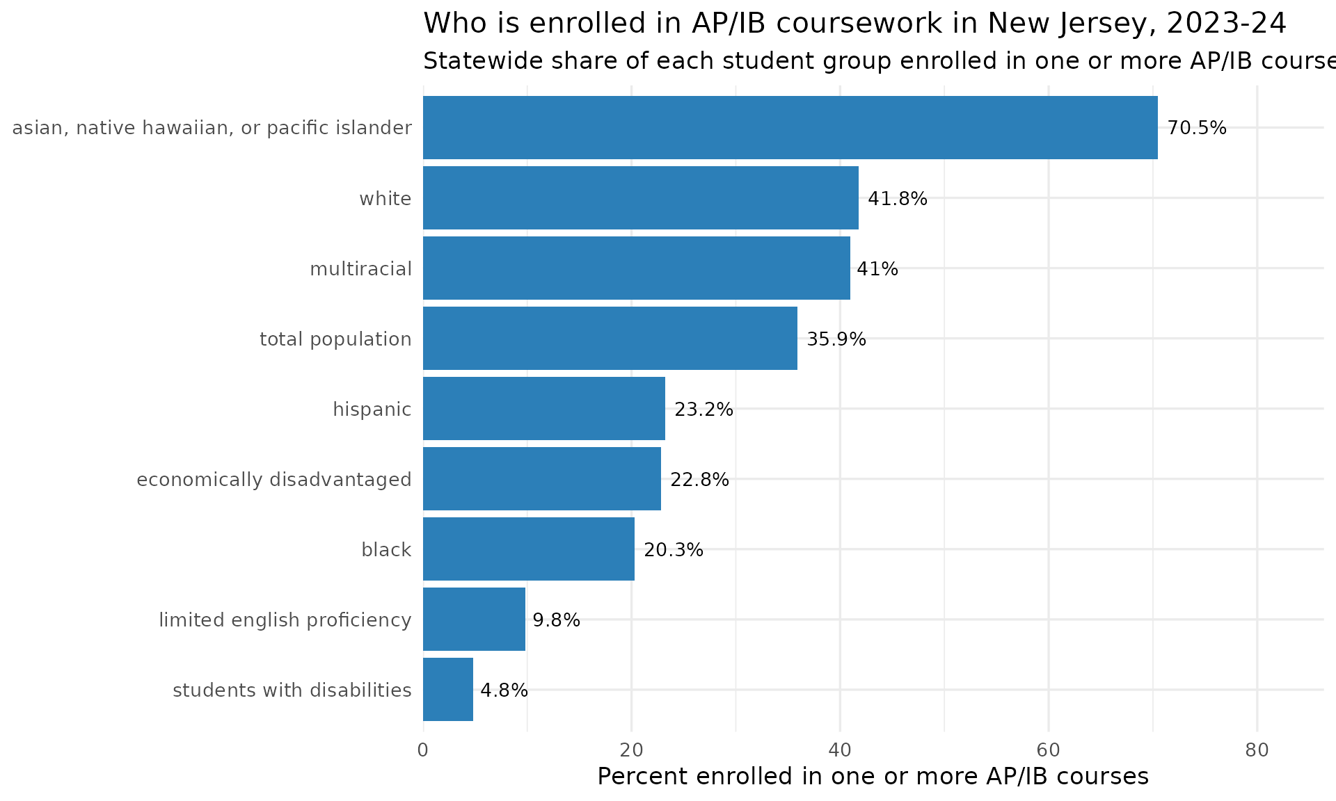
How many advanced courses does a school offer at all?
Access starts with supply. type = "courses_offered"
lists every advanced course a school runs, so counting distinct courses
per school measures the breadth of the advanced-course
menu. In 2023-24 the typical NJ high school offering any advanced course
listed about 19 of them, but the range is enormous - from a single
course to nearly 50.
breadth <- fetch_advanced_course_access(2024, type = "courses_offered") %>%
  filter(is_school) %>%
  group_by(district_id, school_id, school_name) %>%
  summarise(n_courses = n_distinct(course_name), .groups = "drop")

# Print-before-plot.
stopifnot(nrow(breadth) > 0)
summary(breadth$n_courses)
#>    Min. 1st Qu.  Median    Mean 3rd Qu.    Max.
#>    2.00   11.00   19.00   18.81   26.00   49.00
ggplot(breadth, aes(x = n_courses)) +
  geom_histogram(binwidth = 2, fill = "#2c7fb8", colour = "white") +
  geom_vline(xintercept = median(breadth$n_courses),
             linetype = "dashed", colour = "#d95f0e", linewidth = 0.9) +
  labs(
    title = "Breadth of the advanced-course menu, 2023-24",
    subtitle = paste0("Distinct AP/IB courses offered per school; dashed line = median (",
                      median(breadth$n_courses), " courses)"),
    x = "Number of distinct advanced courses offered",
    y = "Number of schools"
  ) +
  theme_minimal(base_size = 13)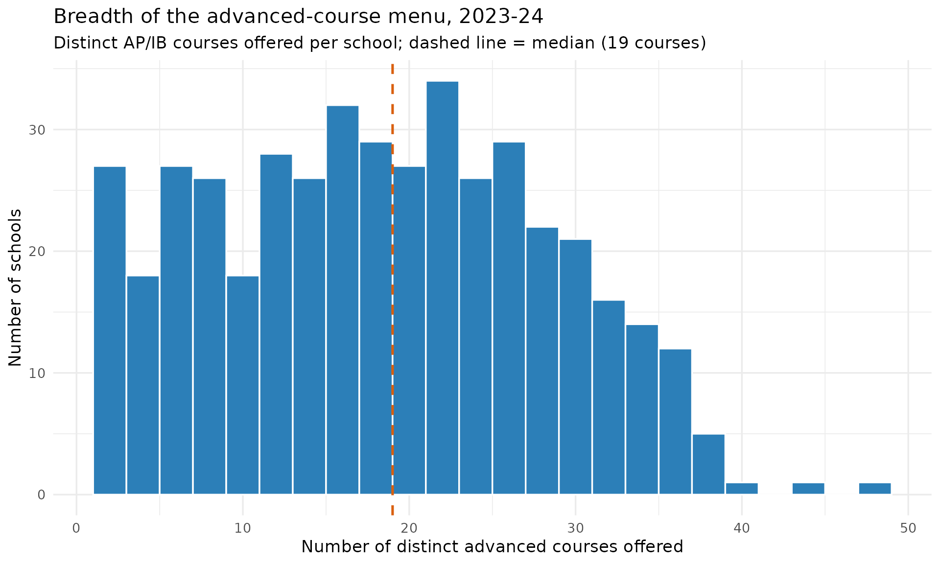
The schools with the widest menus:
breadth %>%
  arrange(desc(n_courses)) %>%
  slice_head(n = 10) %>%
  select(school_name, n_courses)
#> # A tibble: 10 × 2
#>    school_name                     n_courses
#>    <chr>                               <int>
#>  1 West Morris Mendham High School        49
#>  2 West Morris Central High School        45
#>  3 Howell High School                     41
#>  4 Morris Knolls High School              39
#>  5 Freehold Township High School          38
#>  6 Livingston High School                 38
#>  7 Randolph High School                   38
#>  8 Red Bank Regional High School          38
#>  9 Bergen County Academies                37
#> 10 Bridgewater-Raritan High School        37
Notes
-
fetch_advanced_course_access()acceptslevel = "school"(default) orlevel = "district"; the statewideis_staterow lives in the District workbook. - Coverage:
courses_offeredandslespan 2017-2025;participation_by_groupspans 2021-2025 (the sheet is absent 2017-2020 and those years error). The 2025 participation sheet is a multi-year trend table filtered to the requested year. - Suppression / no-data strings (e.g. “There is no data available for
this school year.”) are coerced to
NA, never a fabricated number.
sessionInfo()
#> R version 4.6.2 (2026-10-29)
#> Platform: x86_64-pc-linux-gnu
#> Running under: Ubuntu 26.04.1 LTS
#>
#> Matrix products: default
#> BLAS:   /usr/lib/x86_64-linux-gnu/openblas-pthread/libblas.so.3
#> LAPACK: /usr/lib/x86_64-linux-gnu/openblas-pthread/libopenblasp-r0.3.32.so;  LAPACK version 3.12.0
#>
#> locale:
#>  [1] LC_CTYPE=C.UTF-8       LC_NUMERIC=C           LC_TIME=C.UTF-8
#>  [4] LC_COLLATE=C.UTF-8     LC_MONETARY=C.UTF-8    LC_MESSAGES=C.UTF-8
#>  [7] LC_PAPER=C.UTF-8       LC_NAME=C              LC_ADDRESS=C
#> [10] LC_TELEPHONE=C         LC_MEASUREMENT=C.UTF-8 LC_IDENTIFICATION=C
#>
#> time zone: UTC
#> tzcode source: system (glibc)
#>
#> attached base packages:
#> [1] stats     graphics  grDevices utils     datasets  methods   base
#>
#> other attached packages:
#> [1] ggplot2_4.0.4       dplyr_1.2.1         njschooldata_0.11.0
#>
#> loaded via a namespace (and not attached):
#>  [1] utf8_1.2.6         rappdirs_0.3.4     sass_0.5.0         generics_0.1.4
#>  [5] tidyr_1.3.2        stringi_1.8.9      hms_1.1.4          digest_0.6.39
#>  [9] magrittr_2.0.5     evaluate_1.0.5     grid_4.6.2         timechange_0.4.0
#> [13] RColorBrewer_1.1-3 fastmap_1.2.0      cellranger_1.1.0   jsonlite_2.0.0
#> [17] purrr_1.2.2        scales_1.4.0       textshaping_1.1.0  jquerylib_0.1.4
#> [21] cli_3.6.6          rlang_1.3.0        withr_3.0.3        cachem_1.1.0
#> [25] yaml_2.3.12        otel_0.3.0         tools_4.6.2        tzdb_0.5.0
#> [29] curl_8.1.0         vctrs_0.7.3        R6_2.6.1           lifecycle_1.0.5
#> [33] lubridate_1.9.5    snakecase_0.11.1   stringr_1.6.0      fs_2.1.0
#> [37] ragg_1.5.2         janitor_2.2.1      pkgconfig_2.0.3    desc_1.4.3
#> [41] pkgdown_2.2.1      pillar_1.11.1      bslib_0.12.0       gtable_0.3.6
#> [45] glue_1.8.1         systemfonts_1.3.3  xfun_0.62          tibble_3.3.1
#> [49] tidyselect_1.2.1   knitr_1.52         farver_2.1.2       htmltools_0.5.9
#> [53] labeling_0.4.3     rmarkdown_2.32     readr_2.2.0        compiler_4.6.2
#> [57] S7_1.0.0           readxl_1.6.0