Overview
This vignette performs data quality checks on New York State school enrollment data from 2012-2024. We examine:
- Statewide enrollment trends (noting year-over-year changes > 5%)
- District-level analysis for 5 major districts
- Data completeness and anomalies
Fetch Multi-Year Data
We retrieve enrollment data for all available years (2012-2024).
# Fetch district-level data for all available years
years <- 2012:2024

# Get enrollment data year by year (handles errors gracefully)
enr_all <- fetch_enr_years(years, level = "district", tidy = TRUE, use_cache = TRUE)
## Downloading district enrollment data for 2012 ...## Cached data for 2012## Downloading district enrollment data for 2013 ...## Cached data for 2013## Downloading district enrollment data for 2014 ...## Cached data for 2014## Downloading district enrollment data for 2015 ...## Cached data for 2015## Downloading district enrollment data for 2016 ...## Cached data for 2016## Downloading district enrollment data for 2017 ...## Cached data for 2017## Downloading district enrollment data for 2018 ...## Cached data for 2018## Downloading district enrollment data for 2019 ...## Cached data for 2019## Downloading district enrollment data for 2020 ...## Cached data for 2020## Downloading district enrollment data for 2021 ...## Cached data for 2021## Downloading district enrollment data for 2022 ...## Cached data for 2022## Downloading district enrollment data for 2023 ...## Cached data for 2023## Downloading district enrollment data for 2024 ...## Cached data for 2024
# Check what years we actually got
years_retrieved <- sort(unique(enr_all$end_year))
message("Years retrieved: ", paste(years_retrieved, collapse = ", "))
## Years retrieved: 2012, 2013, 2014, 2015, 2016, 2017, 2018, 2019, 2020, 2021, 2022, 2023, 2024Statewide Enrollment Trends
Total State Enrollment by Year
state_totals <- enr_all %>%
  filter(grade_level == "TOTAL") %>%
  group_by(end_year) %>%
  summarize(
    total_enrollment = sum(n_students, na.rm = TRUE),
    n_districts = n_distinct(district_code),
    .groups = "drop"
  ) %>%
  arrange(end_year) %>%
  mutate(
    yoy_change = total_enrollment - lag(total_enrollment),
    yoy_pct = yoy_change / lag(total_enrollment) * 100,
    flag_large_change = abs(yoy_pct) > 5
  )

state_totals
## # A tibble: 13 × 6
## end_year total_enrollment n_districts yoy_change yoy_pct flag_large_change
## <int> <dbl> <int> <dbl> <dbl> <lgl>
## 1 2012 2699840 1 NA NA NA
## 2 2013 2680170 1 -19670 -0.729 FALSE
## 3 2014 2661609 1 -18561 -0.693 FALSE
## 4 2015 2655264 1 -6345 -0.238 FALSE
## 5 2016 2642186 1 -13078 -0.493 FALSE
## 6 2017 2623867 1 -18319 -0.693 FALSE
## 7 2018 2607282 1 -16585 -0.632 FALSE
## 8 2019 2577890 1 -29392 -1.13 FALSE
## 9 2020 2561821 1 -16069 -0.623 FALSE
## 10 2021 2455261 1 -106560 -4.16 FALSE
## 11 2022 2418631 1 -36630 -1.49 FALSE
## 12 2023 2403931 718 -14700 -0.608 FALSE
## 13 2024 2404319 718 388 0.0161 FALSEIdentify Large Year-Over-Year Changes
Changes greater than 5% warrant investigation:
large_changes <- state_totals %>%
  filter(flag_large_change == TRUE)

if (nrow(large_changes) > 0) {
  message("WARNING: Found ", nrow(large_changes), " year(s) with >5% enrollment change:")
  print(large_changes %>% select(end_year, total_enrollment, yoy_pct))
} else {
  message("No year-over-year changes exceeded 5% threshold")
}
## No year-over-year changes exceeded 5% thresholdStatewide Trend Visualization
ggplot(state_totals, aes(x = end_year, y = total_enrollment)) +
  geom_line(linewidth = 1, color = "steelblue") +
  geom_point(size = 2.5, color = "steelblue") +
  geom_point(
    data = state_totals %>% filter(flag_large_change),
    aes(x = end_year, y = total_enrollment),
    color = "red", size = 4
  ) +
  scale_y_continuous(labels = comma, limits = c(0, NA)) +
  scale_x_continuous(breaks = years_retrieved) +
  labs(
    title = "New York State Total Public School Enrollment",
    subtitle = "Red points indicate >5% year-over-year change",
    x = "School Year (End Year)",
    y = "Total Enrollment",
    caption = "Source: NYSED IRS Public School Enrollment"
  ) +
  theme_minimal() +
  theme(
    axis.text.x = element_text(angle = 45, hjust = 1),
    plot.title = element_text(face = "bold")
  )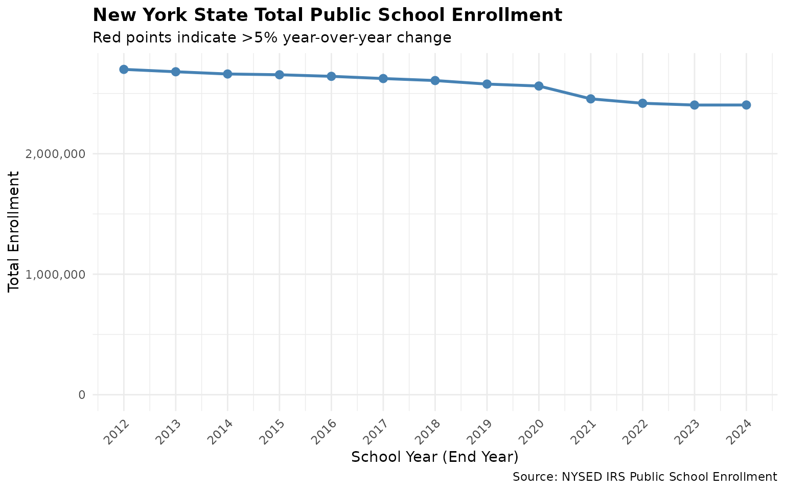
NY State Total Public School Enrollment
Year-Over-Year Percentage Change
ggplot(
  state_totals %>% filter(!is.na(yoy_pct)),
  aes(x = end_year, y = yoy_pct)
) +
  geom_col(
    aes(fill = yoy_pct > 0),
    show.legend = FALSE
  ) +
  geom_hline(yintercept = c(-5, 5), linetype = "dashed", color = "red") +
  scale_fill_manual(values = c("TRUE" = "steelblue", "FALSE" = "coral")) +
  scale_x_continuous(breaks = years_retrieved[-1]) +
  labs(
    title = "Year-Over-Year Enrollment Change (%)",
    subtitle = "Dashed lines show +/- 5% threshold",
    x = "School Year (End Year)",
    y = "Percentage Change"
  ) +
  theme_minimal() +
  theme(axis.text.x = element_text(angle = 45, hjust = 1))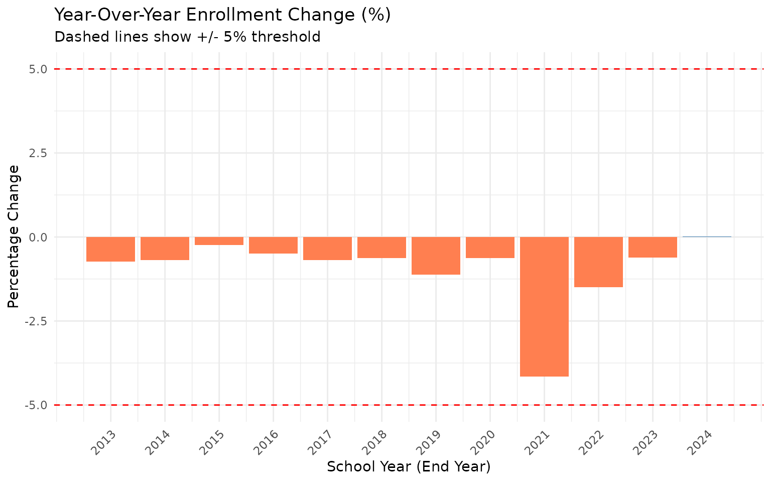
Year-over-year percentage change in enrollment
Major District Analysis
We examine 5 major NY districts:
- NYC DOE - New York City Department of Education (district code starting with “31”)
- Buffalo City SD - Second largest district
- Rochester City SD - Third largest district
- Yonkers Public Schools - Fourth largest district
- Syracuse City SD - Fifth largest district
# Major district codes (first 6 digits of BEDS code)
major_districts <- tribble(
  ~district_code, ~district_label,
  "310200", "NYC DOE",
  "140600", "Buffalo City SD",
  "261600", "Rochester City SD",
  "662300", "Yonkers Public Schools",
  "421800", "Syracuse City SD"
)

# Note: NYC has multiple district_code prefixes (31xxxx)
# Let's identify the actual codes in our data

# Find NYC districts
nyc_districts <- enr_all %>%
  filter(is_nyc, grade_level == "TOTAL") %>%
  distinct(district_code, district_name) %>%
  head(5)

message("NYC district codes found:")
## NYC district codes found:
print(nyc_districts)## district_code district_name
## 1 307500 NYC SPEC SCHOOLS - DIST 75
## 2 310100 NYC GEOG DIST # 1 - MANHATTAN
## 3 310200 NYC GEOG DIST # 2 - MANHATTAN
## 4 310300 NYC GEOG DIST # 3 - MANHATTAN
## 5 310400 NYC GEOG DIST # 4 - MANHATTAN
# Find other major districts by name
all_districts <- enr_all %>%
  filter(grade_level == "TOTAL") %>%
  distinct(district_code, district_name)

# Search for our target districts
buffalo <- all_districts %>% filter(grepl("BUFFALO", toupper(district_name)))
rochester <- all_districts %>% filter(grepl("ROCHESTER", toupper(district_name)))
yonkers <- all_districts %>% filter(grepl("YONKERS", toupper(district_name)))
syracuse <- all_districts %>% filter(grepl("SYRACUSE", toupper(district_name)))

message("\nDistrict codes found:")
##
## District codes found:## Buffalo: NA, 140600## Rochester: NA, NA, 261313, 261600## Yonkers: NA, 662300## Syracuse: NA, NA, NA, 420303, 420401, 421800District-Level Enrollment Trends
# Combine district codes for filtering
# NYC is special - aggregate all 31xxxx districts
target_districts <- c(
  buffalo$district_code[1],
  rochester$district_code[1],
  yonkers$district_code[1],
  syracuse$district_code[1]
)

# Get NYC aggregate
nyc_trend <- enr_all %>%
  filter(is_nyc, grade_level == "TOTAL") %>%
  group_by(end_year) %>%
  summarize(
    n_students = sum(n_students, na.rm = TRUE),
    .groups = "drop"
  ) %>%
  mutate(district_label = "NYC DOE")

# Get other major districts
other_trends <- enr_all %>%
  filter(
    district_code %in% target_districts,
    grade_level == "TOTAL"
  ) %>%
  select(end_year, district_name, n_students) %>%
  mutate(district_label = case_when(
    grepl("BUFFALO", toupper(district_name)) ~ "Buffalo City SD",
    grepl("ROCHESTER", toupper(district_name)) ~ "Rochester City SD",
    grepl("YONKERS", toupper(district_name)) ~ "Yonkers Public Schools",
    grepl("SYRACUSE", toupper(district_name)) ~ "Syracuse City SD",
    TRUE ~ district_name
  )) %>%
  select(end_year, district_label, n_students)

# Combine
district_trends <- bind_rows(nyc_trend, other_trends)

district_trends
## # A tibble: 7,932 × 3
## end_year n_students district_label
## <int> <dbl> <chr>
## 1 2023 895097 NYC DOE
## 2 2024 898410 NYC DOE
## 3 2012 8495 ALBANY
## 4 2012 927 BERNE KNOX
## 5 2012 4936 BETHLEHEM
## 6 2012 2036 RAVENA COEYMANS
## 7 2012 1972 COHOES
## 8 2012 5231 SOUTH COLONIE
## 9 2012 256 MENANDS
## 10 2012 5512 NORTH COLONIE CSD
## # ℹ 7,922 more rowsDistrict Enrollment Visualization
# Calculate YoY changes by district
district_yoy <- district_trends %>%
  arrange(district_label, end_year) %>%
  group_by(district_label) %>%
  mutate(
    yoy_pct = (n_students - lag(n_students)) / lag(n_students) * 100,
    flag_change = abs(yoy_pct) > 5
  ) %>%
  ungroup()

# Plot
ggplot(district_yoy, aes(x = end_year, y = n_students, color = district_label)) +
  geom_line(linewidth = 1) +
  geom_point(size = 2) +
  geom_point(
    data = district_yoy %>% filter(flag_change == TRUE),
    size = 4, shape = 1, stroke = 1.5
  ) +
  scale_y_continuous(labels = comma) +
  scale_x_continuous(breaks = years_retrieved) +
  scale_color_brewer(palette = "Set1") +
  labs(
    title = "Enrollment Trends: Major NY Districts",
    subtitle = "Circled points indicate >5% year-over-year change",
    x = "School Year (End Year)",
    y = "Total Enrollment",
    color = "District",
    caption = "Source: NYSED IRS Public School Enrollment"
  ) +
  theme_minimal() +
  theme(
    axis.text.x = element_text(angle = 45, hjust = 1),
    legend.position = "bottom"
  ) +
  guides(color = guide_legend(nrow = 2))
## Warning in RColorBrewer::brewer.pal(n, pal): n too large, allowed maximum for palette Set1 is 9
## Returning the palette you asked for with that many colors## Warning: Removed 7851 rows containing missing values or values outside the scale range
## (`geom_line()`).## Warning: Removed 7851 rows containing missing values or values outside the scale range
## (`geom_point()`).## Warning: Removed 1528 rows containing missing values or values outside the scale range
## (`geom_point()`).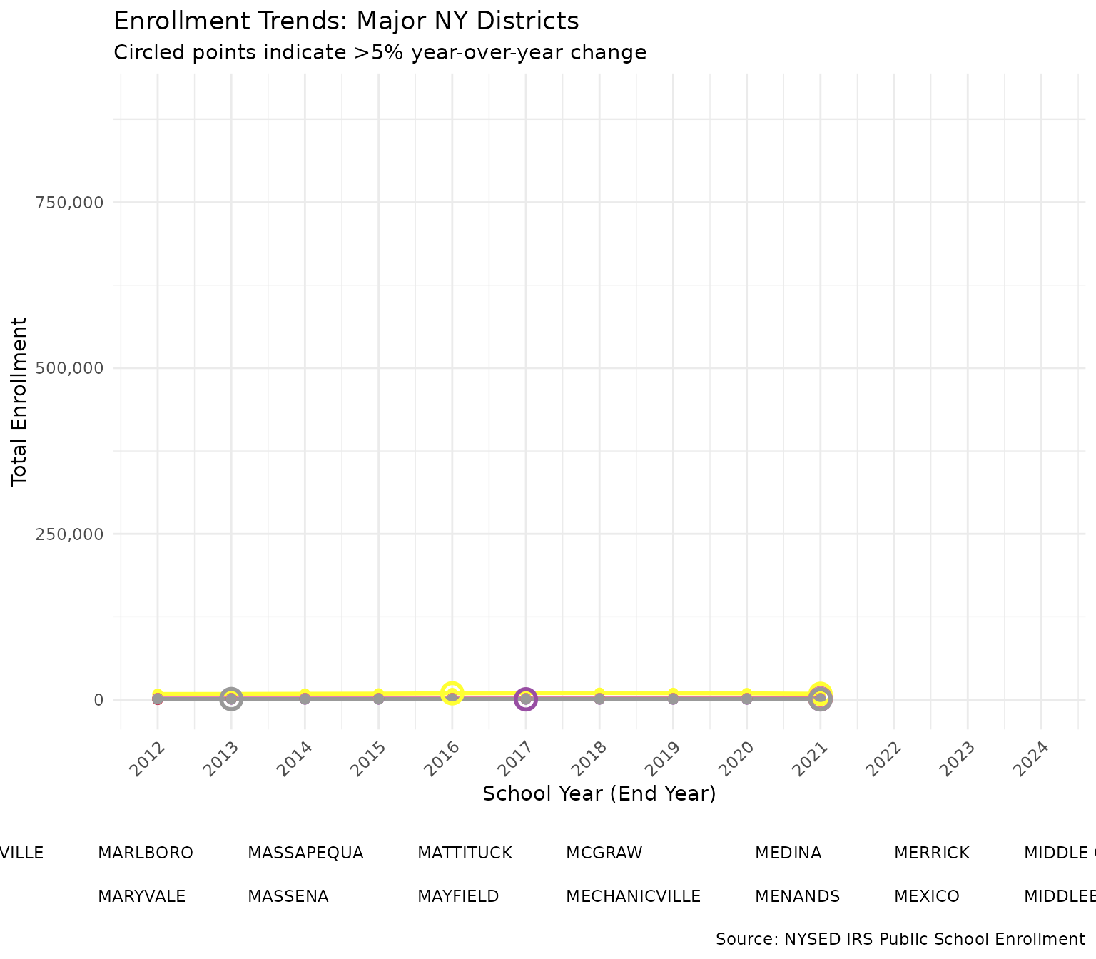
Major district enrollment trends
District-Level Large Changes
district_flags <- district_yoy %>%
  filter(flag_change == TRUE) %>%
  arrange(district_label, end_year) %>%
  select(district_label, end_year, n_students, yoy_pct)

if (nrow(district_flags) > 0) {
  message("Districts with >5% YoY changes:")
  print(district_flags)
} else {
  message("No major districts had >5% year-over-year changes")
}
## Districts with >5% YoY changes:## # A tibble: 1,537 × 4
## district_label end_year n_students yoy_pct
## <chr> <int> <dbl> <dbl>
## 1 AFTON 2017 513 -5.70
## 2 AFTON 2021 481 -7.85
## 3 AKRON 2021 1282 -7.50
## 4 ALBANY 2016 9625 6.00
## 5 ALBANY 2021 8853 -7.28
## 6 ALBION 2021 1783 -5.01
## 7 ALDEN 2021 1527 -6.43
## 8 ALEXANDER 2013 879 -5.89
## 9 ALEXANDER 2021 759 -7.66
## 10 ALEXANDRIA CSD 2015 574 -7.27
## # ℹ 1,527 more rowsDistrict Enrollment Table
# Wide table of enrollment by district and year
district_wide <- district_trends %>%
  tidyr::pivot_wider(
    names_from = end_year,
    values_from = n_students
  )
## Warning: Values from `n_students` are not uniquely identified; output will contain
## list-cols.
## • Use `values_fn = list` to suppress this warning.
## • Use `values_fn = {summary_fun}` to summarise duplicates.
## • Use the following dplyr code to identify duplicates.
## {data} |>
## dplyr::summarise(n = dplyr::n(), .by = c(district_label, end_year)) |>
## dplyr::filter(n > 1L)
district_wide## # A tibble: 730 × 14
## district_label `2023` `2024` `2012` `2013` `2014` `2015` `2016` `2017` `2018`
## <chr> <list> <list> <list> <list> <list> <list> <list> <list> <list>
## 1 NYC DOE <dbl> <dbl> <NULL> <NULL> <NULL> <NULL> <NULL> <NULL> <NULL>
## 2 ALBANY <NULL> <NULL> <dbl> <dbl> <dbl> <dbl> <dbl> <dbl> <dbl>
## 3 BERNE KNOX <NULL> <NULL> <dbl> <dbl> <dbl> <dbl> <dbl> <dbl> <dbl>
## 4 BETHLEHEM <NULL> <NULL> <dbl> <dbl> <dbl> <dbl> <dbl> <dbl> <dbl>
## 5 RAVENA COEYMA… <NULL> <NULL> <dbl> <dbl> <dbl> <dbl> <dbl> <dbl> <dbl>
## 6 COHOES <NULL> <NULL> <dbl> <dbl> <dbl> <dbl> <dbl> <dbl> <dbl>
## 7 SOUTH COLONIE <NULL> <NULL> <dbl> <dbl> <dbl> <dbl> <dbl> <dbl> <dbl>
## 8 MENANDS <NULL> <NULL> <dbl> <dbl> <dbl> <dbl> <dbl> <dbl> <dbl>
## 9 NORTH COLONIE… <NULL> <NULL> <dbl> <dbl> <dbl> <dbl> <dbl> <dbl> <dbl>
## 10 GREEN ISLAND <NULL> <NULL> <dbl> <dbl> <dbl> <dbl> <dbl> <dbl> <dbl>
## # ℹ 720 more rows
## # ℹ 4 more variables: `2019` <list>, `2020` <list>, `2021` <list>,
## # `2022` <list>Data Completeness Checks
Missing Data by Year
missing_summary <- enr_all %>%
  filter(grade_level == "TOTAL") %>%
  group_by(end_year) %>%
  summarize(
    n_districts = n_distinct(district_code),
    n_missing_enrollment = sum(is.na(n_students)),
    pct_missing = n_missing_enrollment / n() * 100,
    .groups = "drop"
  )

missing_summary
## # A tibble: 13 × 4
## end_year n_districts n_missing_enrollment pct_missing
## <int> <int> <int> <dbl>
## 1 2012 1 0 0
## 2 2013 1 0 0
## 3 2014 1 0 0
## 4 2015 1 0 0
## 5 2016 1 0 0
## 6 2017 1 0 0
## 7 2018 1 0 0
## 8 2019 1 0 0
## 9 2020 1 0 0
## 10 2021 1 0 0
## 11 2022 1 0 0
## 12 2023 718 0 0
## 13 2024 718 0 0Grade-Level Data Availability
Check which grade levels are available across years:
grade_avail <- enr_all %>%
  group_by(end_year, grade_level) %>%
  summarize(
    n_records = n(),
    n_with_data = sum(!is.na(n_students)),
    .groups = "drop"
  ) %>%
  filter(grade_level %in% c("TOTAL", "K", "01", "05", "09", "12"))

tidyr::pivot_wider(
  grade_avail,
  id_cols = end_year,
  names_from = grade_level,
  values_from = n_with_data
)
## # A tibble: 13 × 7
## end_year `01` `05` `09` `12` TOTAL K
## <int> <int> <int> <int> <int> <int> <int>
## 1 2012 726 726 726 726 726 NA
## 2 2013 723 723 723 723 723 NA
## 3 2014 721 721 721 721 721 NA
## 4 2015 721 721 721 721 721 NA
## 5 2016 721 721 721 721 721 NA
## 6 2017 721 721 721 721 721 NA
## 7 2018 721 721 721 721 721 NA
## 8 2019 721 721 721 721 721 NA
## 9 2020 719 719 719 719 719 NA
## 10 2021 718 718 718 718 718 NA
## 11 2022 718 718 718 718 718 NA
## 12 2023 718 718 718 718 718 718
## 13 2024 718 718 718 718 718 718Data Quality Issues Found
Based on the analysis above, document any issues:
issues <- list()

# Check for years with large statewide changes
if (nrow(large_changes) > 0) {
  issues$statewide_jumps <- large_changes$end_year
}

# Check for district-level anomalies
if (nrow(district_flags) > 0) {
  issues$district_anomalies <- district_flags
}

# Check for missing data
high_missing <- missing_summary %>% filter(pct_missing > 1)
if (nrow(high_missing) > 0) {
  issues$high_missing_years <- high_missing$end_year
}

# Print summary
message("\n=== DATA QUALITY SUMMARY ===\n")
##
## === DATA QUALITY SUMMARY ===
if (length(issues) == 0) {
  message("No significant data quality issues identified.")
} else {
  if (!is.null(issues$statewide_jumps)) {
    message("Statewide enrollment jumps (>5%) in years: ",
            paste(issues$statewide_jumps, collapse = ", "))
  }
  if (!is.null(issues$district_anomalies)) {
    message("\nDistrict-level anomalies:")
    print(issues$district_anomalies)
  }
  if (!is.null(issues$high_missing_years)) {
    message("\nYears with >1% missing data: ",
            paste(issues$high_missing_years, collapse = ", "))
  }
}
##
## District-level anomalies:## # A tibble: 1,537 × 4
## district_label end_year n_students yoy_pct
## <chr> <int> <dbl> <dbl>
## 1 AFTON 2017 513 -5.70
## 2 AFTON 2021 481 -7.85
## 3 AKRON 2021 1282 -7.50
## 4 ALBANY 2016 9625 6.00
## 5 ALBANY 2021 8853 -7.28
## 6 ALBION 2021 1783 -5.01
## 7 ALDEN 2021 1527 -6.43
## 8 ALEXANDER 2013 879 -5.89
## 9 ALEXANDER 2021 759 -7.66
## 10 ALEXANDRIA CSD 2015 574 -7.27
## # ℹ 1,527 more rowsRecommendations
Based on this QA analysis:
Statewide trends: Review any years flagged with >5% changes to determine if they represent genuine enrollment shifts or data collection issues.
District analysis: Major urban districts (NYC, Buffalo, Rochester, Yonkers, Syracuse) should be monitored for unusual year-over-year changes.
Data completeness: Years with high missing data rates may need special handling in analyses.
Session Info
## R version 4.5.2 (2025-10-31)
## Platform: x86_64-pc-linux-gnu
## Running under: Ubuntu 24.04.3 LTS
##
## Matrix products: default
## BLAS:   /usr/lib/x86_64-linux-gnu/openblas-pthread/libblas.so.3
## LAPACK: /usr/lib/x86_64-linux-gnu/openblas-pthread/libopenblasp-r0.3.26.so;  LAPACK version 3.12.0
##
## locale:
##  [1] LC_CTYPE=C.UTF-8       LC_NUMERIC=C           LC_TIME=C.UTF-8
##  [4] LC_COLLATE=C.UTF-8     LC_MONETARY=C.UTF-8    LC_MESSAGES=C.UTF-8
##  [7] LC_PAPER=C.UTF-8       LC_NAME=C              LC_ADDRESS=C
## [10] LC_TELEPHONE=C         LC_MEASUREMENT=C.UTF-8 LC_IDENTIFICATION=C
##
## time zone: UTC
## tzcode source: system (glibc)
##
## attached base packages:
## [1] stats     graphics  grDevices utils     datasets  methods   base
##
## other attached packages:
## [1] scales_1.4.0       ggplot2_4.0.2      dplyr_1.2.0        nyschooldata_0.1.0
##
## loaded via a namespace (and not attached):
##  [1] gtable_0.3.6       jsonlite_2.0.0     compiler_4.5.2     tidyselect_1.2.1
##  [5] tidyr_1.3.2        jquerylib_0.1.4    systemfonts_1.3.2  textshaping_1.0.5
##  [9] readxl_1.4.5       yaml_2.3.12        fastmap_1.2.0      R6_2.6.1
## [13] labeling_0.4.3     generics_0.1.4     knitr_1.51         tibble_3.3.1
## [17] desc_1.4.3         downloader_0.4.1   bslib_0.10.0       pillar_1.11.1
## [21] RColorBrewer_1.1-3 rlang_1.1.7        utf8_1.2.6         cachem_1.1.0
## [25] xfun_0.56          fs_1.6.7           sass_0.4.10        S7_0.2.1
## [29] cli_3.6.5          pkgdown_2.2.0      withr_3.0.2        magrittr_2.0.4
## [33] digest_0.6.39      grid_4.5.2         rappdirs_0.3.4     lifecycle_1.0.5
## [37] vctrs_0.7.1        evaluate_1.0.5     glue_1.8.0         cellranger_1.1.0
## [41] farver_2.1.2       codetools_0.2-20   ragg_1.5.1         purrr_1.2.1
## [45] rmarkdown_2.30     tools_4.5.2        pkgconfig_2.0.3    htmltools_0.5.9