library(okschooldata)
library(dplyr)
library(tidyr)
library(ggplot2)
theme_set(theme_minimal(base_size = 14))
Oklahoma educates over 700,000 students across 543 school districts – one of the most fragmented systems in the nation. This vignette explores enrollment trends using data from the Oklahoma State Department of Education (OSDE) for school years 2015-16 through 2022-23.
Data note: Years 2018, 2020, 2024, and 2025 have parser issues with OSDE file format changes and are excluded from multi-year analyses. Only years with verified clean data are used: 2016, 2017, 2019, 2021, 2022, 2023.
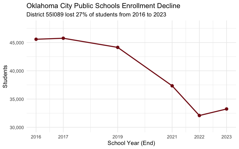
1. Oklahoma City Lost 27% of Its Students Since 2016
Oklahoma City Public Schools (55I089) shed over 12,000 students from 2016 to 2023, a decline of 27.1% – the steepest drop of any large Oklahoma district. The district went from being the state’s largest to trading places with Tulsa.
enr_multi <- fetch_enr_multi(c(2016, 2017, 2019, 2021, 2022, 2023), use_cache = TRUE)

okc_trend <- enr_multi |>
  filter(is_district, district_id == "55I089",
         subgroup == "total_enrollment", grade_level == "TOTAL") |>
  select(end_year, district_name, n_students) |>
  arrange(end_year)

stopifnot(nrow(okc_trend) > 0)
print(okc_trend)
#>   end_year district_name n_students
#> 1     2016 OKLAHOMA CITY      45577
#> 2     2017 OKLAHOMA CITY      45757
#> 3     2019 OKLAHOMA CITY      44138
#> 4     2021 OKLAHOMA CITY      37344
#> 5     2022 OKLAHOMA CITY      32086
#> 6     2023 OKLAHOMA CITY      33245

ggplot(okc_trend, aes(x = end_year, y = n_students)) +
  geom_line(linewidth = 1.2, color = "#841617") +
  geom_point(size = 3, color = "#841617") +
  scale_y_continuous(labels = scales::comma, limits = c(30000, 48000)) +
  scale_x_continuous(breaks = c(2016, 2017, 2019, 2021, 2022, 2023)) +
  labs(
    title = "Oklahoma City Public Schools Enrollment Decline",
    subtitle = "District 55I089 lost 27% of students from 2016 to 2023",
    x = "School Year (End)",
    y = "Students"
  )
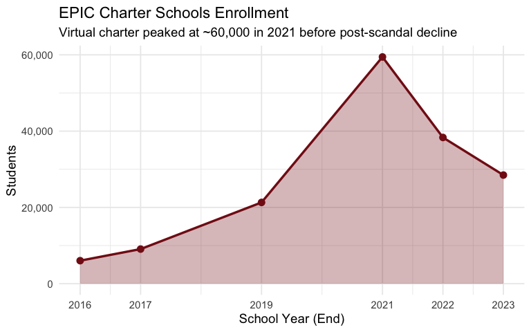
2. EPIC Charter Schools: From 6,000 to 60,000 and Back
EPIC Charter Schools (virtual) grew from 6,037 students in 2016 to a staggering 59,445 in 2021, making it the largest educational entity in Oklahoma. After a financial scandal and state audit, enrollment fell back to 28,478 by 2023.
epic_trend <- enr_multi |>
  filter(is_district, grepl("EPIC|Epic", district_name, ignore.case = TRUE),
         subgroup == "total_enrollment", grade_level == "TOTAL") |>
  group_by(end_year) |>
  summarize(n_students = sum(n_students), .groups = "drop") |>
  arrange(end_year)

stopifnot(nrow(epic_trend) > 0)
print(epic_trend)
#> # A tibble: 6 × 2
#>   end_year n_students
#>      <dbl>      <dbl>
#> 1     2016       6037
#> 2     2017       9077
#> 3     2019      21305
#> 4     2021      59445
#> 5     2022      38334
#> 6     2023      28478

ggplot(epic_trend, aes(x = end_year, y = n_students)) +
  geom_area(fill = "#841617", alpha = 0.3) +
  geom_line(color = "#841617", linewidth = 1.2) +
  geom_point(color = "#841617", size = 3) +
  scale_y_continuous(labels = scales::comma, limits = c(0, NA)) +
  scale_x_continuous(breaks = c(2016, 2017, 2019, 2021, 2022, 2023)) +
  labs(
    title = "EPIC Charter Schools Enrollment",
    subtitle = "Virtual charter peaked at ~60,000 in 2021 before post-scandal decline",
    x = "School Year (End)",
    y = "Students"
  )
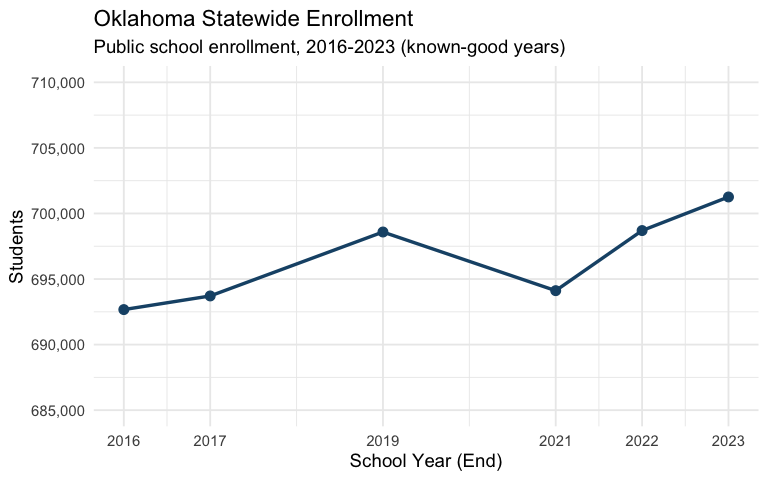
3. Statewide Enrollment Grew Modestly Despite Urban Losses
Despite OKC’s 27% decline, statewide enrollment grew from 692,670 to 701,258 between 2016 and 2023 – a modest 1.2% gain. Suburban growth and charter expansion offset urban losses.
state_trend <- enr_multi |>
  filter(is_state, subgroup == "total_enrollment", grade_level == "TOTAL") |>
  select(end_year, n_students) |>
  arrange(end_year)

stopifnot(nrow(state_trend) > 0)
print(state_trend)
#>   end_year n_students
#> 1     2016     692670
#> 2     2017     693710
#> 3     2019     698586
#> 4     2021     694113
#> 5     2022     698696
#> 6     2023     701258

ggplot(state_trend, aes(x = end_year, y = n_students)) +
  geom_line(linewidth = 1.2, color = "#1a5276") +
  geom_point(size = 3, color = "#1a5276") +
  scale_y_continuous(labels = scales::comma, limits = c(685000, 710000)) +
  scale_x_continuous(breaks = c(2016, 2017, 2019, 2021, 2022, 2023)) +
  labs(
    title = "Oklahoma Statewide Enrollment",
    subtitle = "Public school enrollment, 2016-2023 (known-good years)",
    x = "School Year (End)",
    y = "Students"
  )
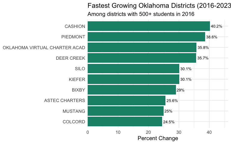
4. Suburban Boomtowns: Piedmont and Deer Creek Lead Growth
Piedmont (+38.6%) and Deer Creek (+35.7%) led enrollment growth among mid-to-large districts from 2016 to 2023. These OKC-area suburban districts absorbed families leaving urban cores.
growth <- enr_multi |>
  filter(is_district, subgroup == "total_enrollment", grade_level == "TOTAL",
         end_year %in% c(2016, 2023)) |>
  select(end_year, district_id, district_name, n_students) |>
  pivot_wider(names_from = end_year, values_from = n_students, names_prefix = "yr_") |>
  filter(!is.na(yr_2016), !is.na(yr_2023), yr_2016 >= 500) |>
  mutate(
    change = yr_2023 - yr_2016,
    pct_change = round(change / yr_2016 * 100, 1)
  ) |>
  arrange(desc(pct_change))

top_growers <- head(growth, 10)
stopifnot(nrow(top_growers) > 0)
print(top_growers |> select(district_name, yr_2016, yr_2023, pct_change))
#> # A tibble: 10 × 4
#>    district_name                 yr_2016 yr_2023 pct_change
#>    <chr>                           <dbl>   <dbl>      <dbl>
#>  1 CASHION                           517     725       40.2
#>  2 PIEDMONT                         3649    5056       38.6
#>  3 OKLAHOMA VIRTUAL CHARTER ACAD    2400    3259       35.8
#>  4 DEER CREEK                       5628    7636       35.7
#>  5 SILO                              889    1157       30.1
#>  6 KIEFER                            731     951       30.1
#>  7 BIXBY                            6046    7800       29
#>  8 ASTEC CHARTERS                    928    1166       25.6
#>  9 MUSTANG                         10798   13494       25
#> 10 COLCORD                           607     756       24.5

ggplot(top_growers,
       aes(x = reorder(district_name, pct_change), y = pct_change)) +
  geom_col(fill = "#148f77") +
  geom_text(aes(label = paste0(pct_change, "%")), hjust = -0.1, size = 3.5) +
  scale_y_continuous(expand = expansion(mult = c(0, 0.15))) +
  coord_flip() +
  labs(
    title = "Fastest Growing Oklahoma Districts (2016-2023)",
    subtitle = "Among districts with 500+ students in 2016",
    x = NULL,
    y = "Percent Change"
  )
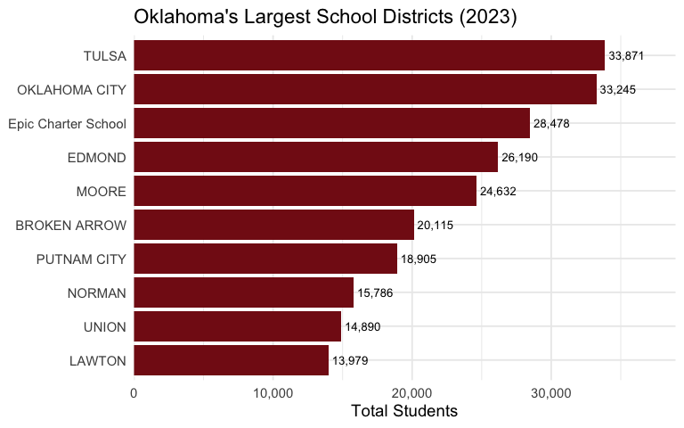
5. Top 10 Districts by Enrollment
Tulsa narrowly edges Oklahoma City as the state’s largest traditional district, while EPIC Charter and Edmond compete for third.
top10 <- enr_multi |>
  filter(is_district, subgroup == "total_enrollment", grade_level == "TOTAL",
         end_year == 2023) |>
  select(district_id, district_name, n_students) |>
  arrange(desc(n_students)) |>
  head(10)

stopifnot(nrow(top10) > 0)
print(top10)
#>    district_id       district_name n_students
#> 1       72I001               TULSA      33871
#> 2       55I089       OKLAHOMA CITY      33245
#> 3       55Z014 Epic Charter School      28478
#> 4       55I012              EDMOND      26190
#> 5       14I002               MOORE      24632
#> 6       72I003        BROKEN ARROW      20115
#> 7       55I001         PUTNAM CITY      18905
#> 8       14I029              NORMAN      15786
#> 9       72I009               UNION      14890
#> 10      16I008              LAWTON      13979

ggplot(top10, aes(x = reorder(district_name, n_students), y = n_students)) +
  geom_col(fill = "#841617") +
  geom_text(aes(label = scales::comma(n_students)), hjust = -0.1, size = 3.5) +
  scale_y_continuous(labels = scales::comma, expand = expansion(mult = c(0, 0.15))) +
  coord_flip() +
  labs(
    title = "Oklahoma's Largest School Districts (2023)",
    x = NULL,
    y = "Total Students"
  )
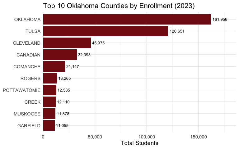
6. Two Counties Hold 40% of All Students
Oklahoma and Tulsa counties together enroll 282,607 students – 40.3% of the entire state.
county_enr <- enr_multi |>
  filter(is_district, grade_level == "TOTAL", subgroup == "total_enrollment",
         end_year == 2023) |>
  group_by(county) |>
  summarize(n_students = sum(n_students, na.rm = TRUE), .groups = "drop") |>
  filter(!is.na(county)) |>
  arrange(desc(n_students)) |>
  head(10)

stopifnot(nrow(county_enr) > 0)
print(county_enr)
#> # A tibble: 10 × 2
#>    county       n_students
#>    <chr>             <dbl>
#>  1 OKLAHOMA         161956
#>  2 TULSA            120651
#>  3 CLEVELAND         45975
#>  4 CANADIAN          32393
#>  5 COMANCHE          21147
#>  6 ROGERS            13265
#>  7 POTTAWATOMIE      12535
#>  8 CREEK             12110
#>  9 MUSKOGEE          11878
#> 10 GARFIELD          11055

ggplot(county_enr, aes(x = reorder(county, n_students), y = n_students)) +
  geom_col(fill = "#841617") +
  geom_text(aes(label = scales::comma(n_students)), hjust = -0.1, size = 3.5) +
  scale_y_continuous(labels = scales::comma, expand = expansion(mult = c(0, 0.15))) +
  coord_flip() +
  labs(
    title = "Top 10 Oklahoma Counties by Enrollment (2023)",
    x = NULL,
    y = "Total Students"
  )
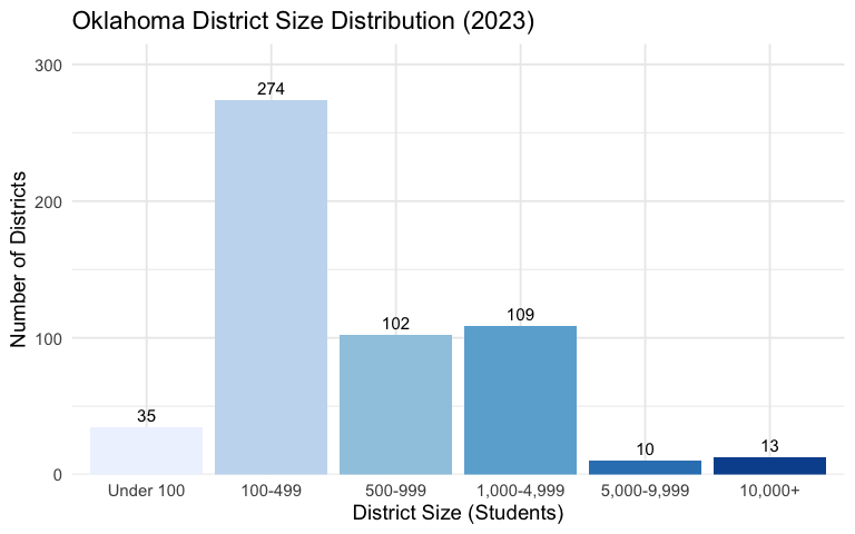
7. 309 Districts Have Fewer Than 500 Students
Oklahoma’s 543 districts include 309 with fewer than 500 students. Only 13 districts top 10,000.
size_dist <- enr_multi |>
  filter(is_district, subgroup == "total_enrollment", grade_level == "TOTAL",
         end_year == 2023) |>
  mutate(
    size_bucket = case_when(
      n_students < 100 ~ "Under 100",
      n_students < 500 ~ "100-499",
      n_students < 1000 ~ "500-999",
      n_students < 5000 ~ "1,000-4,999",
      n_students < 10000 ~ "5,000-9,999",
      TRUE ~ "10,000+"
    ),
    size_bucket = factor(size_bucket,
      levels = c("Under 100", "100-499", "500-999",
                 "1,000-4,999", "5,000-9,999", "10,000+"))
  ) |>
  count(size_bucket)

stopifnot(nrow(size_dist) > 0)
print(size_dist)
#>   size_bucket   n
#> 1   Under 100  35
#> 2     100-499 274
#> 3     500-999 102
#> 4 1,000-4,999 109
#> 5 5,000-9,999  10
#> 6     10,000+  13

ggplot(size_dist, aes(x = size_bucket, y = n, fill = size_bucket)) +
  geom_col(show.legend = FALSE) +
  geom_text(aes(label = n), vjust = -0.5, size = 4) +
  scale_y_continuous(expand = expansion(mult = c(0, 0.15))) +
  scale_fill_brewer(palette = "Blues") +
  labs(
    title = "Oklahoma District Size Distribution (2023)",
    x = "District Size (Students)",
    y = "Number of Districts"
  )
8. Southeast Oklahoma Is Shrinking
The 10 southeastern counties (McCurtain, Pushmataha, Choctaw, LeFlore, Latimer, Pittsburg, Atoka, Bryan, Coal, Haskell) lost 3.7% of enrollment while the rest of the state grew 1.5%.
se_counties <- c("MCCURTAIN", "PUSHMATAHA", "CHOCTAW", "LEFLORE", "LATIMER",
                 "PITTSBURG", "ATOKA", "BRYAN", "COAL", "HASKELL")

region_trend <- enr_multi |>
  filter(is_district, subgroup == "total_enrollment", grade_level == "TOTAL") |>
  mutate(region = if_else(county %in% se_counties, "Southeast", "Rest of State")) |>
  group_by(end_year, region) |>
  summarize(n_students = sum(n_students), .groups = "drop") |>
  group_by(region) |>
  mutate(index = round(n_students / first(n_students) * 100, 1)) |>
  ungroup()

stopifnot(nrow(region_trend) > 0)
print(region_trend)
#> # A tibble: 12 × 4
#>    end_year region        n_students index
#>       <dbl> <chr>              <dbl> <dbl>
#>  1     2016 Rest of State     657935 100
#>  2     2016 Southeast          34735 100
#>  3     2017 Rest of State     659040 100.
#>  4     2017 Southeast          34670  99.8
#>  5     2019 Rest of State     664703 101
#>  6     2019 Southeast          33883  97.5
#>  7     2021 Rest of State     662068 101.
#>  8     2021 Southeast          32045  92.3
#>  9     2022 Rest of State     665768 101.
#> 10     2022 Southeast          32928  94.8
#> 11     2023 Rest of State     667791 102.
#> 12     2023 Southeast          33467  96.3

ggplot(region_trend, aes(x = end_year, y = index, color = region)) +
  geom_hline(yintercept = 100, linetype = "dashed", color = "gray50") +
  geom_line(linewidth = 1) +
  geom_point(size = 2) +
  scale_x_continuous(breaks = c(2016, 2017, 2019, 2021, 2022, 2023)) +
  scale_color_manual(values = c("Southeast" = "#841617", "Rest of State" = "#1a5276")) +
  labs(
    title = "Southeast Oklahoma vs. Rest of State",
    subtitle = "Enrollment index: 2016 = 100",
    x = "School Year (End)",
    y = "Index (2016 = 100)",
    color = NULL
  ) +
  theme(legend.position = "bottom")
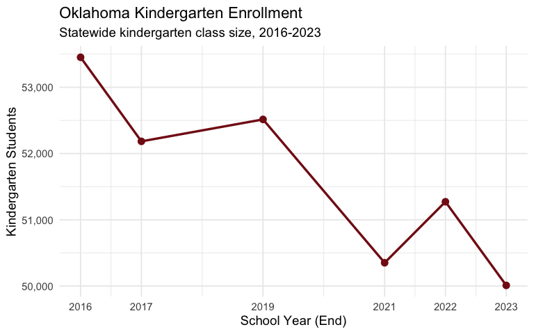
9. Kindergarten Enrollment Dropped 6% Since 2016
Kindergarten enrollment fell from 53,453 in 2016 to 50,009 in 2023. The COVID-era dip in 2021 (50,351) barely recovered.
k_trend <- enr_multi |>
  filter(is_state, subgroup == "total_enrollment", grade_level == "K") |>
  select(end_year, n_students) |>
  arrange(end_year)

stopifnot(nrow(k_trend) > 0)
print(k_trend)
#>   end_year n_students
#> 1     2016      53453
#> 2     2017      52184
#> 3     2019      52515
#> 4     2021      50351
#> 5     2022      51272
#> 6     2023      50009

ggplot(k_trend, aes(x = end_year, y = n_students)) +
  geom_line(color = "#841617", linewidth = 1.2) +
  geom_point(color = "#841617", size = 3) +
  scale_y_continuous(labels = scales::comma) +
  scale_x_continuous(breaks = c(2016, 2017, 2019, 2021, 2022, 2023)) +
  labs(
    title = "Oklahoma Kindergarten Enrollment",
    subtitle = "Statewide kindergarten class size, 2016-2023",
    x = "School Year (End)",
    y = "Kindergarten Students"
  )
10. Tulsa and OKC Follow the Same Downward Path
Both Tulsa (72I001) and Oklahoma City (55I089) experienced parallel enrollment declines since 2016, losing students to suburban districts and virtual schools.
urban_trend <- enr_multi |>
  filter(is_district, district_id %in% c("55I089", "72I001"),
         subgroup == "total_enrollment", grade_level == "TOTAL") |>
  mutate(district_label = case_when(
    district_id == "55I089" ~ "Oklahoma City",
    district_id == "72I001" ~ "Tulsa"
  )) |>
  select(end_year, district_label, n_students)

stopifnot(nrow(urban_trend) > 0)
print(urban_trend)
#>    end_year district_label n_students
#> 1      2016  Oklahoma City      45577
#> 2      2016          Tulsa      40867
#> 3      2017  Oklahoma City      45757
#> 4      2017          Tulsa      40459
#> 5      2019  Oklahoma City      44138
#> 6      2019          Tulsa      39056
#> 7      2021  Oklahoma City      37344
#> 8      2021          Tulsa      35765
#> 9      2022  Oklahoma City      32086
#> 10     2022          Tulsa      33211
#> 11     2023  Oklahoma City      33245
#> 12     2023          Tulsa      33871

ggplot(urban_trend, aes(x = end_year, y = n_students, color = district_label)) +
  geom_line(linewidth = 1) +
  geom_point(size = 2) +
  scale_y_continuous(labels = scales::comma) +
  scale_x_continuous(breaks = c(2016, 2017, 2019, 2021, 2022, 2023)) +
  scale_color_manual(values = c("Oklahoma City" = "#841617", "Tulsa" = "#1a5276")) +
  labs(
    title = "Tulsa and OKC: Parallel Urban Decline",
    subtitle = "Both districts lost ~20-27% of enrollment since 2016",
    x = "School Year (End)",
    y = "Students",
    color = "District"
  ) +
  theme(legend.position = "bottom")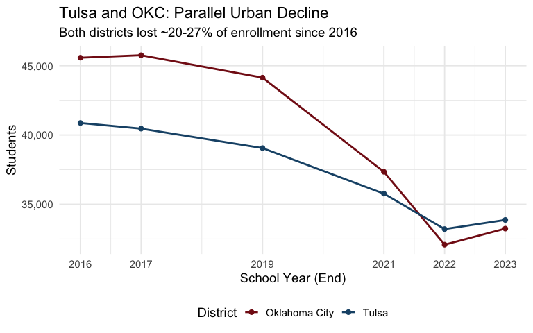
Summary
Oklahoma’s enrollment story is defined by:
- Urban flight: OKC lost 27%, Tulsa lost 17%, as families moved to suburbs and virtual schools
- Virtual school explosion: EPIC Charter went from 6K to 60K before declining after scandal
- Suburban boom: Piedmont, Deer Creek, and Bixby are the state’s fastest-growing districts
- Fragmentation: 309 of 543 districts have fewer than 500 students
- Geographic concentration: Oklahoma and Tulsa counties hold 40% of all students
- Regional decline: Southeast Oklahoma is losing students faster than the rest of the state
- Shrinking kindergarten: K enrollment dropped 6% since 2016
Use fetch_enr() and fetch_enr_multi() to
explore these patterns further.
sessionInfo()
#> R version 4.5.2 (2025-10-31)
#> Platform: x86_64-pc-linux-gnu
#> Running under: Ubuntu 24.04.3 LTS
#>
#> Matrix products: default
#> BLAS:   /usr/lib/x86_64-linux-gnu/openblas-pthread/libblas.so.3
#> LAPACK: /usr/lib/x86_64-linux-gnu/openblas-pthread/libopenblasp-r0.3.26.so;  LAPACK version 3.12.0
#>
#> locale:
#>  [1] LC_CTYPE=C.UTF-8       LC_NUMERIC=C           LC_TIME=C.UTF-8
#>  [4] LC_COLLATE=C.UTF-8     LC_MONETARY=C.UTF-8    LC_MESSAGES=C.UTF-8
#>  [7] LC_PAPER=C.UTF-8       LC_NAME=C              LC_ADDRESS=C
#> [10] LC_TELEPHONE=C         LC_MEASUREMENT=C.UTF-8 LC_IDENTIFICATION=C
#>
#> time zone: UTC
#> tzcode source: system (glibc)
#>
#> attached base packages:
#> [1] stats     graphics  grDevices utils     datasets  methods   base
#>
#> other attached packages:
#> [1] ggplot2_4.0.2      tidyr_1.3.2        dplyr_1.2.0        okschooldata_0.1.0
#>
#> loaded via a namespace (and not attached):
#>  [1] gtable_0.3.6       jsonlite_2.0.0     compiler_4.5.2     tidyselect_1.2.1
#>  [5] jquerylib_0.1.4    systemfonts_1.3.2  scales_1.4.0       textshaping_1.0.5
#>  [9] readxl_1.4.5       yaml_2.3.12        fastmap_1.2.0      R6_2.6.1
#> [13] labeling_0.4.3     generics_0.1.4     curl_7.0.0         knitr_1.51
#> [17] tibble_3.3.1       desc_1.4.3         bslib_0.10.0       pillar_1.11.1
#> [21] RColorBrewer_1.1-3 rlang_1.1.7        utf8_1.2.6         cachem_1.1.0
#> [25] xfun_0.56          fs_1.6.7           sass_0.4.10        S7_0.2.1
#> [29] cli_3.6.5          withr_3.0.2        pkgdown_2.2.0      magrittr_2.0.4
#> [33] digest_0.6.39      grid_4.5.2         rappdirs_0.3.4     lifecycle_1.0.5
#> [37] vctrs_0.7.1        evaluate_1.0.5     glue_1.8.0         cellranger_1.1.0
#> [41] farver_2.1.2       codetools_0.2-20   ragg_1.5.1         httr_1.4.8
#> [45] rmarkdown_2.30     purrr_1.2.1        tools_4.5.2        pkgconfig_2.0.3
#> [49] htmltools_0.5.9