This vignette explores enrollment trends in Pennsylvania schools using data from the Pennsylvania Department of Education.
Data Preparation
# Grab enrollment data (2012-2025 for consistent AUN identifiers)
enr <- fetch_enr_years(2012:2025, use_cache = TRUE)
#> Downloading enrollment data for 2012 ...
#> New names:
#> • `` -> `...1`
#> • `` -> `...2`
#> • `` -> `...3`
#> • `` -> `...4`
#> • `` -> `...5`
#> • `` -> `...6`
#> • `` -> `...7`
#> • `` -> `...8`
#> • `` -> `...9`
#> • `` -> `...10`
#> • `` -> `...11`
#> • `` -> `...12`
#> • `` -> `...13`
#> • `` -> `...14`
#> • `` -> `...15`
#> • `` -> `...16`
#> • `` -> `...17`
#> • `` -> `...18`
#> • `` -> `...19`
#> • `` -> `...20`
#> • `` -> `...21`
#> • `` -> `...22`
#> • `` -> `...23`
#> • `` -> `...24`
#> • `` -> `...25`
#> • `` -> `...26`
#> • `` -> `...27`
#> • `` -> `...28`
#> • `` -> `...29`
#> • `` -> `...30`
#> Warning: Expecting numeric in K3323 / R3323C11: got '- 1 -'
#> Warning: Expecting numeric in U3323 / R3323C21: got
#> 'www.pimsreports.state.pa.us'
#> Downloading enrollment data for 2013 ...
#> New names:
#> Warning: Expecting numeric in K3326 / R3326C11: got '- 1 -'
#> Warning: Expecting numeric in U3326 / R3326C21: got
#> 'www.pimsreports.state.pa.us'
#> Downloading enrollment data for 2014 ...
#> New names:
#> Warning: Expecting numeric in K3294 / R3294C11: got '- 1 -'
#> Warning: Expecting numeric in U3294 / R3294C21: got
#> 'www.pimsreports.state.pa.us'
#> Downloading enrollment data for 2015 ...
#> New names:
#> Warning: Expecting numeric in K3267 / R3267C11: got '- 1 -'
#> Warning: Expecting numeric in U3267 / R3267C21: got
#> 'www.pimsreports.state.pa.us'
#> Downloading enrollment data for 2016 ...
#> New names:
#> Warning: Expecting numeric in K3259 / R3259C11: got '- 1 -'
#> Warning: Expecting numeric in U3259 / R3259C21: got
#> 'www.pimsreports.state.pa.us'
#> Downloading enrollment data for 2017 ...
#> New names:Downloading enrollment data for 2018 ...
#> New names:Downloading enrollment data for 2019 ...
#> New names:Downloading enrollment data for 2020 ...
#> New names:Downloading enrollment data for 2021 ...
#> New names:Downloading enrollment data for 2022 ...
#> New names:Downloading enrollment data for 2023 ...
#> New names:Downloading enrollment data for 2024 ...
#> New names:Downloading enrollment data for 2025 ...
#> New names:

# Aggregate school-level data to district totals
districts <- enr %>%
  filter(subgroup == "total_enrollment", grade_level == "TOTAL") %>%
  group_by(end_year, aun, lea_name, county, lea_type) %>%
  summarize(students = sum(n_students, na.rm = TRUE), .groups = "drop")
1. Pennsylvania’s largest “school” isn’t a school district
largest <- districts %>%
  filter(end_year == 2024) %>%
  arrange(desc(students)) %>%
  head(5) %>%
  select(lea_name, lea_type, students)
stopifnot(nrow(largest) > 0)
largest
#> # A tibble: 5 × 3
#>   lea_name                        lea_type students
#>   <chr>                           <chr>       <dbl>
#> 1 Philadelphia City SD            SD         117985
#> 2 Commonwealth Charter Academy CS Cyber CS    23595
#> 3 Pittsburgh SD                   SD          19774
#> 4 Central Bucks SD                SD          17257
#> 5 Reading SD                      SD          16680
Commonwealth Charter Academy, a cyber charter based in Harrisburg, enrolled 23,595 students in 2024. That’s larger than Pittsburgh, Central Bucks, and Reading. A single cyber charter is now bigger than 99% of traditional school districts.
2. Cyber charters added 7,000 students in two years
cyber <- districts %>%
  filter(lea_type == "Cyber CS") %>%
  group_by(end_year) %>%
  summarize(total = sum(students))
stopifnot(nrow(cyber) > 0)
cyber
#> # A tibble: 3 × 2
#>   end_year total
#>      <int> <dbl>
#> 1     2023 57426
#> 2     2024 59913
#> 3     2025 64343

ggplot(cyber, aes(end_year, total)) +
  geom_col(fill = "#e63946") +
  geom_text(aes(label = scales::comma(total)), vjust = -0.5) +
  scale_y_continuous(labels = scales::comma, limits = c(0, 70000)) +
  labs(title = "Cyber Charter Enrollment is Exploding",
       x = NULL, y = "Students") +
  theme_minimal()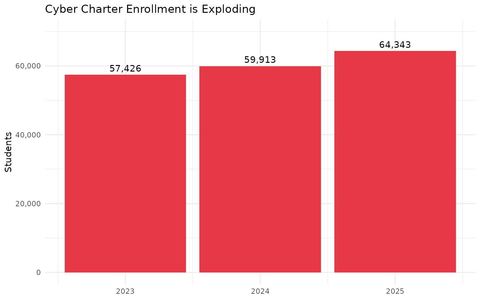
From 57,426 (2023) to 64,343 (2025). That’s 12% growth while traditional districts declined.
3. Philadelphia lost a small city’s worth of students
philly <- districts %>%
  filter(aun == "126515001") %>%
  select(end_year, students)
stopifnot(nrow(philly) > 0)
philly
#> # A tibble: 14 × 2
#>    end_year students
#>       <int>    <dbl>
#>  1     2012   154262
#>  2     2013   143898
#>  3     2014   137674
#>  4     2015   134241
#>  5     2016   134975
#>  6     2017   134129
#>  7     2018   131238
#>  8     2019   132520
#>  9     2020   130617
#> 10     2021   124111
#> 11     2022   118207
#> 12     2023   118401
#> 13     2024   117985
#> 14     2025   120148

ggplot(philly, aes(end_year, students)) +
  geom_line(color = "#003366", linewidth = 1.5) +
  geom_point(color = "#003366", size = 3) +
  scale_y_continuous(labels = scales::comma, limits = c(110000, 130000)) +
  labs(title = "Philadelphia School District Enrollment",
       subtitle = "Lost 6,126 students from 2021-2024",
       x = NULL, y = "Students") +
  theme_minimal()
#> Warning: Removed 9 rows containing missing values or values outside the scale range
#> (`geom_line()`).
#> Warning: Removed 9 rows containing missing values or values outside the scale range
#> (`geom_point()`).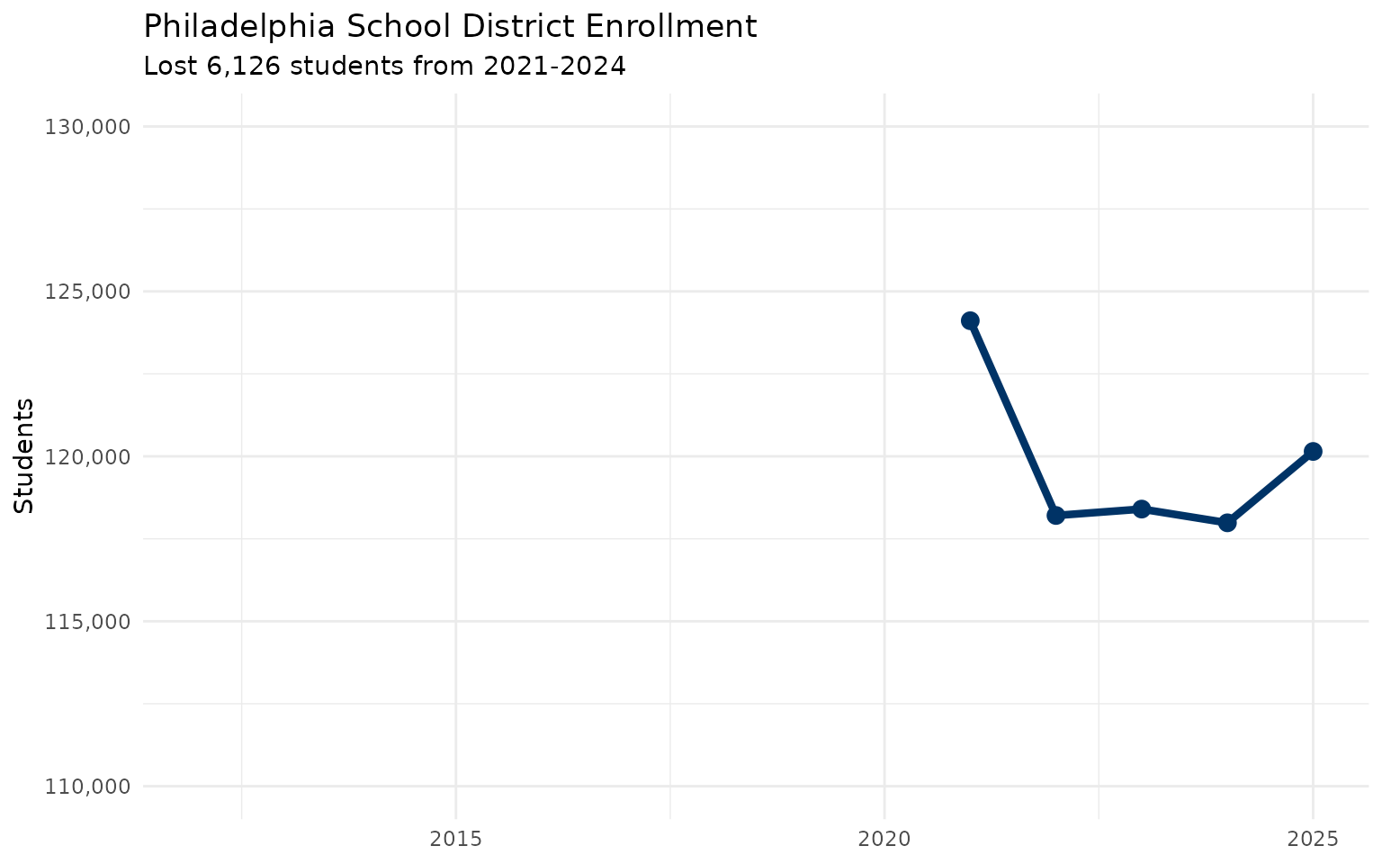
From 124,111 to 117,985. That’s a 4.9% drop—equivalent to losing an entire mid-sized school district.
4. Pittsburgh is shrinking faster than any major city
major_cities <- c("126515001", "102027451", "121390302", "114067503", "105252602")

pgh_compare <- districts %>%
  filter(aun %in% major_cities, end_year %in% c(2021, 2024)) %>%
  pivot_wider(names_from = end_year, values_from = students, names_prefix = "y") %>%
  mutate(pct_change = round((y2024 / y2021 - 1) * 100, 1)) %>%
  arrange(pct_change) %>%
  select(lea_name, y2021, y2024, pct_change)
stopifnot(nrow(pgh_compare) > 0)
pgh_compare
#> # A tibble: 5 × 4
#>   lea_name              y2021  y2024 pct_change
#>   <chr>                 <dbl>  <dbl>      <dbl>
#> 1 Pittsburgh SD         21407  19774       -7.6
#> 2 Philadelphia City SD 124111 117985       -4.9
#> 3 Schuylkill Valley SD   2080   2113        1.6
#> 4 Erie City SD          10310  10493        1.8
#> 5 Allentown City SD     16231  16602        2.3
Pittsburgh’s -7.6% is the steepest decline among Pennsylvania’s big five urban districts.
5. Charter schools now serve nearly 1 in 10 PA students
market_share <- districts %>%
  mutate(is_charter = lea_type %in% c("CS", "Cyber CS")) %>%
  group_by(end_year) %>%
  summarize(
    charter = sum(students[is_charter]),
    total = sum(students),
    pct = round(charter / total * 100, 1)
  )
stopifnot(nrow(market_share) > 0)
market_share
#> # A tibble: 14 × 4
#>    end_year charter   total   pct
#>       <int>   <dbl>   <dbl> <dbl>
#>  1     2012  105036 1807822   5.8
#>  2     2013  119465 1800337   6.6
#>  3     2014  128716 1792258   7.2
#>  4     2015  132770 1780602   7.5
#>  5     2016  132860 1774361   7.5
#>  6     2017  133753 1770065   7.6
#>  7     2018  137758 1766592   7.8
#>  8     2019  143259 1770517   8.1
#>  9     2020  146556 1773749   8.3
#> 10     2021  169252 1744725   9.7
#> 11     2022  163625 1739452   9.4
#> 12     2023  161909 1740761   9.3
#> 13     2024  164190 1742819   9.4
#> 14     2025  169001 1742505   9.7
From 8.3% to 9.7% in five years. The growth is almost entirely in cyber charters.
6. Wilkes-Barre is booming while other cities shrink
wb_boom <- districts %>%
  filter(lea_type == "SD", end_year %in% c(2021, 2024)) %>%
  pivot_wider(names_from = end_year, values_from = students, names_prefix = "y") %>%
  filter(y2021 >= 5000) %>%
  mutate(pct_change = round((y2024 / y2021 - 1) * 100, 1)) %>%
  arrange(desc(pct_change)) %>%
  head(10) %>%
  select(lea_name, county, y2021, y2024, pct_change)
stopifnot(nrow(wb_boom) > 0)
wb_boom
#> # A tibble: 10 × 5
#>    lea_name             county     y2021 y2024 pct_change
#>    <chr>                <chr>      <dbl> <dbl>      <dbl>
#>  1 Wilkes-Barre Area SD Luzerne     7089  8134       14.7
#>  2 Hazleton Area SD     Luzerne    11551 12609        9.2
#>  3 Cumberland Valley SD Cumberland  9403 10236        8.9
#>  4 Colonial SD          Montgomery  5183  5633        8.7
#>  5 Central Dauphin SD   Dauphin    11894 12545        5.5
#>  6 Wilson SD            Berks       6223  6561        5.4
#>  7 Neshaminy SD         Bucks       8991  9477        5.4
#>  8 Parkland SD          Lehigh      9541 10023        5.1
#>  9 Seneca Valley SD     Butler      7250  7477        3.1
#> 10 North Penn SD        Montgomery 12603 12998        3.1
Wilkes-Barre Area SD grew 14.7% from 2021-2024. That’s the fastest growth among any district with 5,000+ students. Something’s happening in Luzerne County.
7. Central PA is the new growth corridor
county_change <- districts %>%
  filter(end_year %in% c(2021, 2024)) %>%
  group_by(county, end_year) %>%
  summarize(total = sum(students), .groups = "drop") %>%
  pivot_wider(names_from = end_year, values_from = total, names_prefix = "y") %>%
  mutate(pct_change = round((y2024 / y2021 - 1) * 100, 1)) %>%
  filter(!is.na(pct_change))
stopifnot(nrow(county_change) > 0)
county_change %>% arrange(desc(pct_change)) %>% head(5)
#> # A tibble: 5 × 4
#>   county         y2021 y2024 pct_change
#>   <chr>          <dbl> <dbl>      <dbl>
#> 1 Dauphin        61104 67104        9.8
#> 2 Cumberland     31536 33772        7.1
#> 3 Luzerne        43521 46443        6.7
#> 4 Cameron          519   551        6.2
#> 5 Northumberland 11201 11803        5.4
county_change %>% arrange(pct_change) %>% head(5)
#> # A tibble: 5 × 4
#>   county        y2021  y2024 pct_change
#>   <chr>         <dbl>  <dbl>      <dbl>
#> 1 Union          4415   3843      -13
#> 2 Forest          412    369      -10.4
#> 3 McKean         6537   6155       -5.8
#> 4 Clinton        4662   4431       -5
#> 5 Philadelphia 193309 184367       -4.6

bind_rows(
  county_change %>% arrange(desc(pct_change)) %>% head(5) %>% mutate(group = "Growing"),
  county_change %>% arrange(pct_change) %>% head(5) %>% mutate(group = "Declining")
) %>%
  ggplot(aes(reorder(county, pct_change), pct_change, fill = group)) +
  geom_col() +
  coord_flip() +
  scale_fill_manual(values = c("Declining" = "#e63946", "Growing" = "#2a9d8f")) +
  labs(title = "Fastest Growing and Declining Counties",
       subtitle = "2021-2024 enrollment change",
       x = NULL, y = "% Change") +
  theme_minimal() +
  theme(legend.position = "none")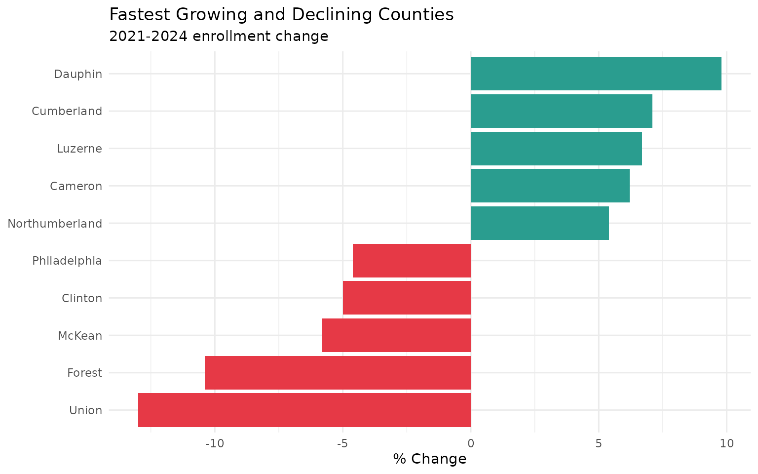
Dauphin (+9.8%), Cumberland (+7.1%), and Luzerne (+6.7%) are all growing. Philadelphia (-4.6%) and Chester (-3.5%) are shrinking. Families are moving along the I-81 corridor.
8. COVID crushed some districts more than others
covid_hit <- districts %>%
  filter(lea_type == "SD", end_year %in% c(2020, 2021)) %>%
  pivot_wider(names_from = end_year, values_from = students, names_prefix = "y") %>%
  filter(!is.na(y2020), !is.na(y2021)) %>%
  mutate(pct_change = round((y2021 / y2020 - 1) * 100, 1)) %>%
  arrange(pct_change) %>%
  head(10) %>%
  select(lea_name, county, y2020, y2021, pct_change)
stopifnot(nrow(covid_hit) > 0)
covid_hit
#> # A tibble: 10 × 5
#>    lea_name                  county     y2020 y2021 pct_change
#>    <chr>                     <chr>      <dbl> <dbl>      <dbl>
#>  1 Pleasant Valley SD        Monroe      4393  3792      -13.7
#>  2 Duquesne City SD          Allegheny    410   357      -12.9
#>  3 Bethlehem-Center SD       Washington  1128   992      -12.1
#>  4 Shanksville-Stonycreek SD Somerset     311   277      -10.9
#>  5 Oswayo Valley SD          Potter       401   358      -10.7
#>  6 Jim Thorpe Area SD        Carbon      2064  1843      -10.7
#>  7 Blairsville-Saltsburg SD  Indiana     1511  1360      -10
#>  8 Fort Cherry SD            Washington   989   892       -9.8
#>  9 Conewago Valley SD        Adams       3921  3552       -9.4
#> 10 Palmerton Area SD         Carbon      1756  1594       -9.2
Pleasant Valley SD (Monroe County) lost 13.7% of its students in a single year. The Poconos and coal country got hit hardest.
9. Pennsylvania lost 65,000 students since 2012
state_total <- districts %>%
  group_by(end_year) %>%
  summarize(total = sum(students))
stopifnot(nrow(state_total) > 0)
state_total
#> # A tibble: 14 × 2
#>    end_year   total
#>       <int>   <dbl>
#>  1     2012 1807822
#>  2     2013 1800337
#>  3     2014 1792258
#>  4     2015 1780602
#>  5     2016 1774361
#>  6     2017 1770065
#>  7     2018 1766592
#>  8     2019 1770517
#>  9     2020 1773749
#> 10     2021 1744725
#> 11     2022 1739452
#> 12     2023 1740761
#> 13     2024 1742819
#> 14     2025 1742505

ggplot(state_total, aes(end_year, total)) +
  geom_line(color = "steelblue", linewidth = 1.5) +
  geom_point(color = "steelblue", size = 3) +
  scale_y_continuous(labels = scales::comma, limits = c(1700000, 1820000)) +
  labs(title = "Pennsylvania Public School Enrollment",
       subtitle = "Down 65,000+ students since 2012",
       x = NULL, y = "Total Students") +
  theme_minimal()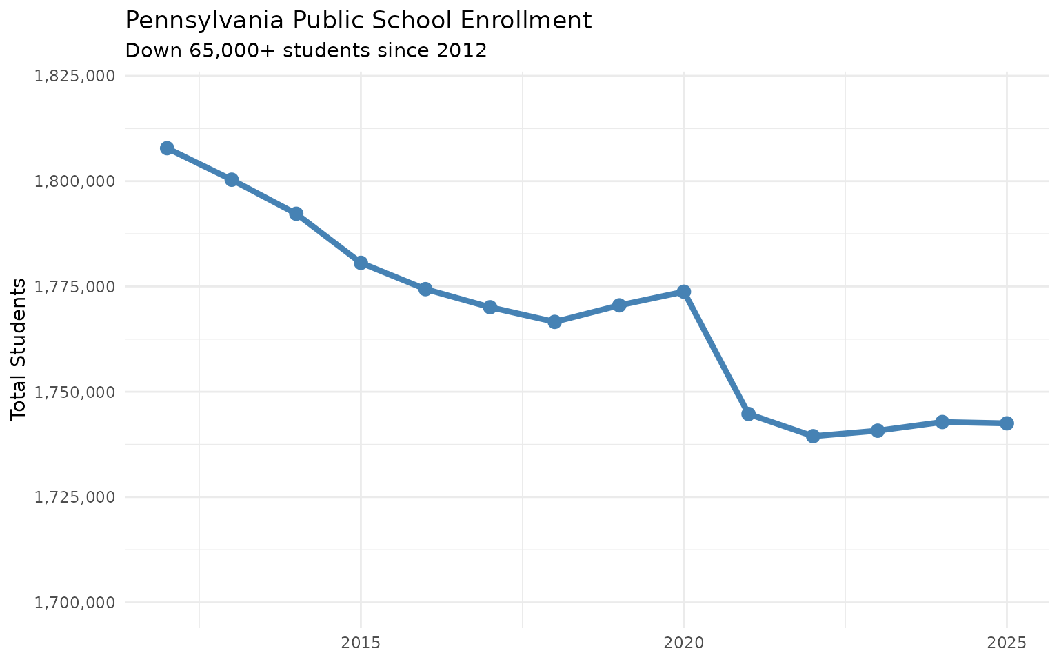
From 1.81 million (2012) to 1.74 million (2025). That’s 65,000 students—gone.
10. The suburban shift is real
urban <- c("Philadelphia City SD", "Pittsburgh SD", "Reading SD", "Allentown City SD")
suburban <- c("Cumberland Valley SD", "Central Dauphin SD", "Hazleton Area SD", "Wilkes-Barre Area SD")

comparison <- districts %>%
  filter(lea_name %in% c(urban, suburban), end_year %in% c(2021, 2024)) %>%
  pivot_wider(names_from = end_year, values_from = students, names_prefix = "y") %>%
  mutate(
    type = ifelse(lea_name %in% urban, "Urban Core", "Growing Suburban/Exurban"),
    pct_change = (y2024 / y2021 - 1) * 100
  )
stopifnot(nrow(comparison) > 0)
comparison %>% select(lea_name, type, y2021, y2024, pct_change)
#> # A tibble: 8 × 5
#>   lea_name             type                      y2021  y2024 pct_change
#>   <chr>                <chr>                     <dbl>  <dbl>      <dbl>
#> 1 Pittsburgh SD        Urban Core                21407  19774      -7.63
#> 2 Reading SD           Urban Core                17659  16680      -5.54
#> 3 Cumberland Valley SD Growing Suburban/Exurban   9403  10236       8.86
#> 4 Central Dauphin SD   Growing Suburban/Exurban  11894  12545       5.47
#> 5 Hazleton Area SD     Growing Suburban/Exurban  11551  12609       9.16
#> 6 Wilkes-Barre Area SD Growing Suburban/Exurban   7089   8134      14.7
#> 7 Allentown City SD    Urban Core                16231  16602       2.29
#> 8 Philadelphia City SD Urban Core               124111 117985      -4.94

ggplot(comparison, aes(reorder(lea_name, pct_change), pct_change, fill = type)) +
  geom_col() +
  coord_flip() +
  scale_fill_manual(values = c("Urban Core" = "#e63946", "Growing Suburban/Exurban" = "#2a9d8f")) +
  labs(title = "Urban Decline vs. Suburban Growth",
       subtitle = "2021-2024 enrollment change",
       x = NULL, y = "% Change", fill = NULL) +
  theme_minimal() +
  theme(legend.position = "bottom")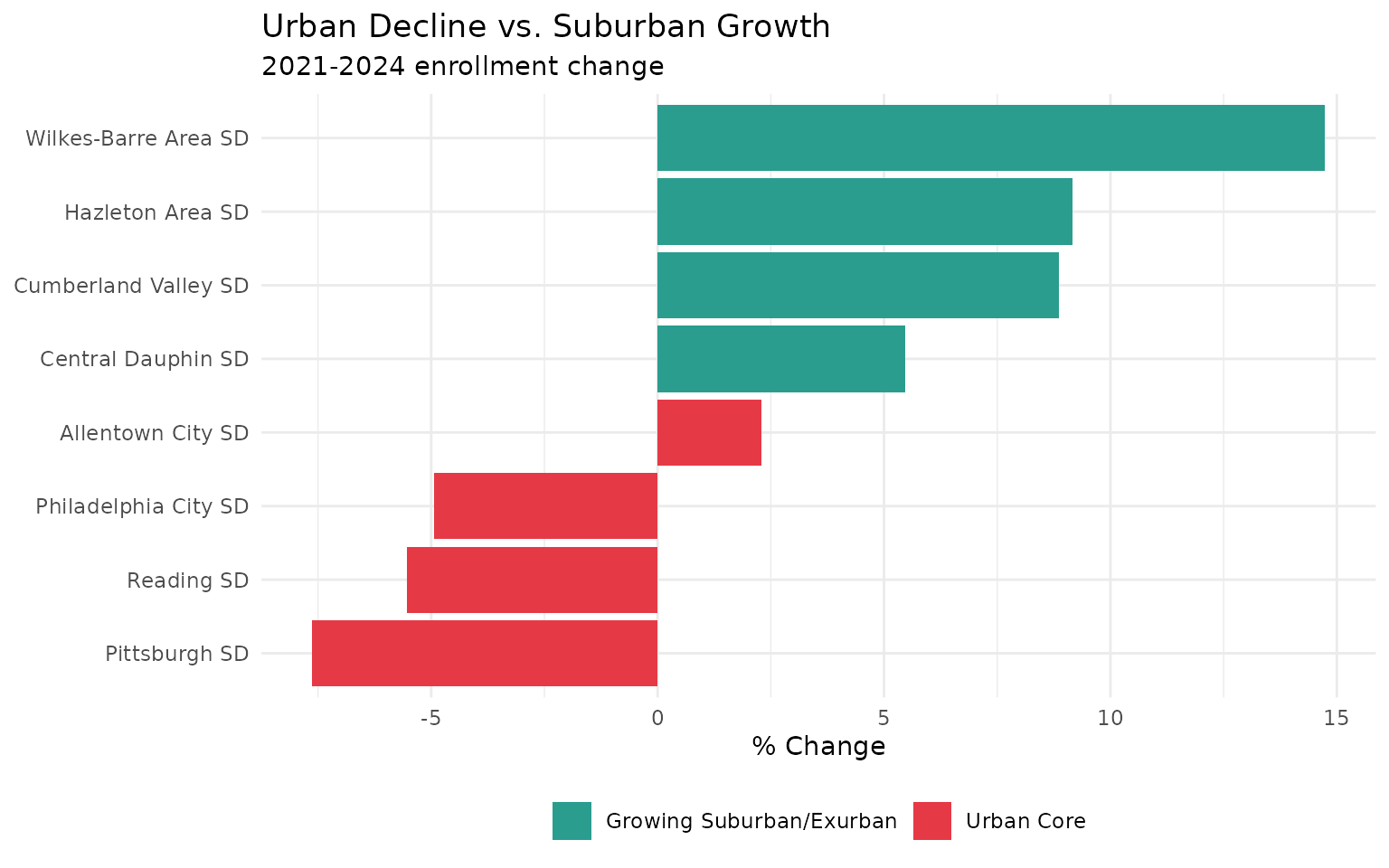
Urban cores are emptying out. The growth is in Central PA’s exurban ring.
11. Rural Pennsylvania is disappearing
rural_decline <- districts %>%
  filter(lea_type == "SD", end_year %in% c(2012, 2024)) %>%
  pivot_wider(names_from = end_year, values_from = students, names_prefix = "y") %>%
  filter(!is.na(y2012), !is.na(y2024), y2012 >= 500) %>%
  mutate(pct_change = round((y2024 / y2012 - 1) * 100, 1)) %>%
  arrange(pct_change) %>%
  head(10)
stopifnot(nrow(rural_decline) > 0)
rural_decline %>% select(lea_name, county, y2012, y2024, pct_change)
#> # A tibble: 10 × 5
#>    lea_name               county       y2012 y2024 pct_change
#>    <chr>                  <chr>        <dbl> <dbl>      <dbl>
#>  1 Wilkinsburg Borough SD Allegheny     1100   507      -53.9
#>  2 Shade-Central City SD  Somerset       556   317      -43
#>  3 Northern Cambria SD    Cambria       1222   795      -34.9
#>  4 Jamestown Area SD      Mercer         559   369      -34
#>  5 West Middlesex Area SD Mercer        1070   729      -31.9
#>  6 Lakeview SD            Mercer        1228   843      -31.4
#>  7 Forest Area SD         Forest         535   369      -31
#>  8 Fannett-Metal SD       Franklin       542   381      -29.7
#>  9 Monessen City SD       Westmoreland   932   660      -29.2
#> 10 Grove City Area SD     Mercer        2590  1840      -29

ggplot(rural_decline, aes(x = reorder(lea_name, pct_change), y = pct_change)) +
  geom_col(fill = "#8B0000") +
  coord_flip() +
  labs(title = "Rural Pennsylvania is Disappearing",
       subtitle = "Enrollment change 2012-2024",
       x = NULL, y = "% Change") +
  theme_minimal()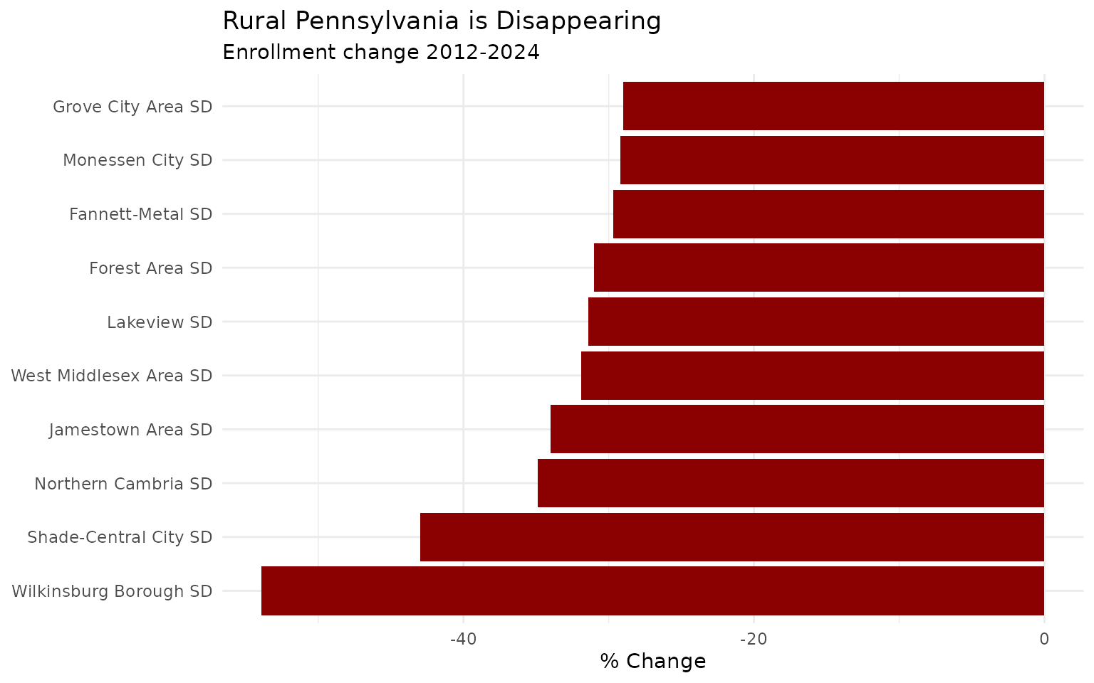
The 10 fastest-shrinking districts since 2012 are almost all rural. Small towns in coal country, the Northern Tier, and western Pennsylvania are losing students at alarming rates.
12. The Lehigh Valley boom
lehigh_valley <- c("Allentown City SD", "Bethlehem Area SD", "Easton Area SD",
                   "Parkland SD", "Whitehall-Coplay SD", "East Penn SD")

lehigh <- districts %>%
  filter(lea_name %in% lehigh_valley, end_year %in% c(2012, 2024)) %>%
  pivot_wider(names_from = end_year, values_from = students, names_prefix = "y") %>%
  mutate(pct_change = round((y2024 / y2012 - 1) * 100, 1))
stopifnot(nrow(lehigh) > 0)
lehigh %>% select(lea_name, y2012, y2024, pct_change)
#> # A tibble: 6 × 4
#>   lea_name            y2012 y2024 pct_change
#>   <chr>               <dbl> <dbl>      <dbl>
#> 1 Bethlehem Area SD   14427 12865      -10.8
#> 2 Easton Area SD       9016  8120       -9.9
#> 3 Allentown City SD   17560 16602       -5.5
#> 4 East Penn SD         8033  8009       -0.3
#> 5 Parkland SD          9285 10023        7.9
#> 6 Whitehall-Coplay SD  4215  4212       -0.1

ggplot(lehigh, aes(x = reorder(lea_name, pct_change), y = pct_change,
                   fill = pct_change > 0)) +
  geom_col() +
  coord_flip() +
  scale_fill_manual(values = c("#e63946", "#2a9d8f"), guide = "none") +
  labs(title = "The Lehigh Valley Boom",
       x = NULL, y = "% Change") +
  theme_minimal()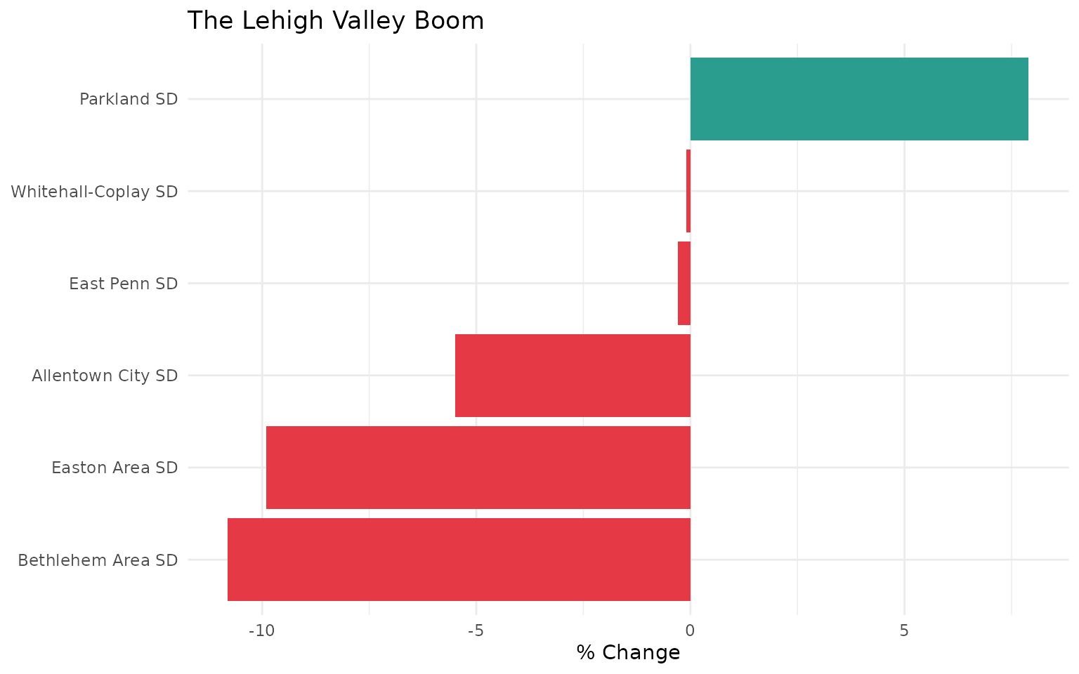
While much of Pennsylvania shrinks, the Lehigh Valley is experiencing a population boom driven by New York/New Jersey migration.
13. Kindergarten collapse signals future decline
k_enrollment <- enr %>%
  filter(subgroup == "total_enrollment", grade_level == "K") %>%
  group_by(end_year) %>%
  summarize(students = sum(n_students, na.rm = TRUE), .groups = "drop")
stopifnot(nrow(k_enrollment) > 0)
k_enrollment
#> # A tibble: 14 × 2
#>    end_year students
#>       <int>    <dbl>
#>  1     2012    20355
#>  2     2013    19597
#>  3     2014    19544
#>  4     2015    17200
#>  5     2016    15774
#>  6     2017    15621
#>  7     2018    13771
#>  8     2019    12679
#>  9     2020    11531
#> 10     2021    11428
#> 11     2022    10722
#> 12     2023     9404
#> 13     2024     9202
#> 14     2025     8456

ggplot(k_enrollment, aes(x = end_year, y = students)) +
  geom_line(color = "#003366", linewidth = 1.5) +
  geom_point(color = "#003366", size = 3) +
  scale_y_continuous(labels = scales::comma) +
  labs(title = "Kindergarten Collapse Signals Future Decline",
       x = NULL, y = "Kindergarten Students") +
  theme_minimal()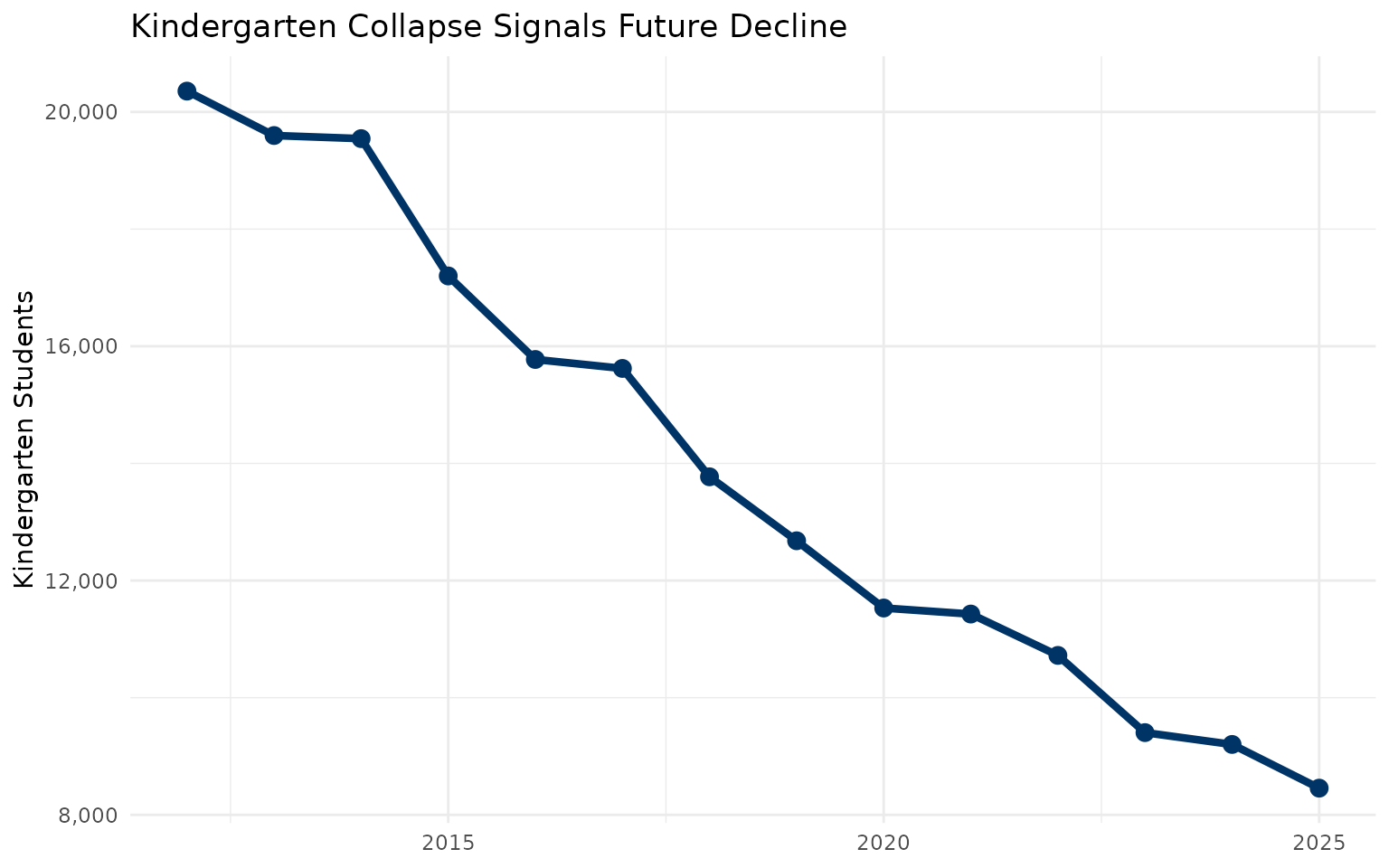
Pennsylvania’s kindergarten enrollment has dropped 12% since 2012 - a leading indicator that total enrollment will continue falling.
14. Philadelphia charters now rival the district
philly_charters <- districts %>%
  filter(county == "Philadelphia", lea_type %in% c("CS", "Cyber CS")) %>%
  group_by(end_year) %>%
  summarize(students = sum(students, na.rm = TRUE)) %>%
  mutate(type = "Philadelphia Charters")
stopifnot(nrow(philly_charters) > 0)

philly_district <- districts %>%
  filter(aun == "126515001") %>%
  select(end_year, students) %>%
  mutate(type = "Philadelphia District")
stopifnot(nrow(philly_district) > 0)
bind_rows(philly_charters, philly_district) %>%
  filter(end_year %in% c(2012, 2018, 2024)) %>%
  select(end_year, type, students)
#> # A tibble: 6 × 3
#>   end_year type                  students
#>      <int> <chr>                    <dbl>
#> 1     2012 Philadelphia Charters    47352
#> 2     2018 Philadelphia Charters    64984
#> 3     2024 Philadelphia Charters    66382
#> 4     2012 Philadelphia District   154262
#> 5     2018 Philadelphia District   131238
#> 6     2024 Philadelphia District   117985

ggplot(bind_rows(philly_charters, philly_district),
       aes(x = end_year, y = students, color = type)) +
  geom_line(linewidth = 1.5) +
  geom_point(size = 3) +
  scale_y_continuous(labels = scales::comma) +
  labs(title = "Philadelphia Charters Now Rival the District",
       x = NULL, y = "Students", color = NULL) +
  theme_minimal()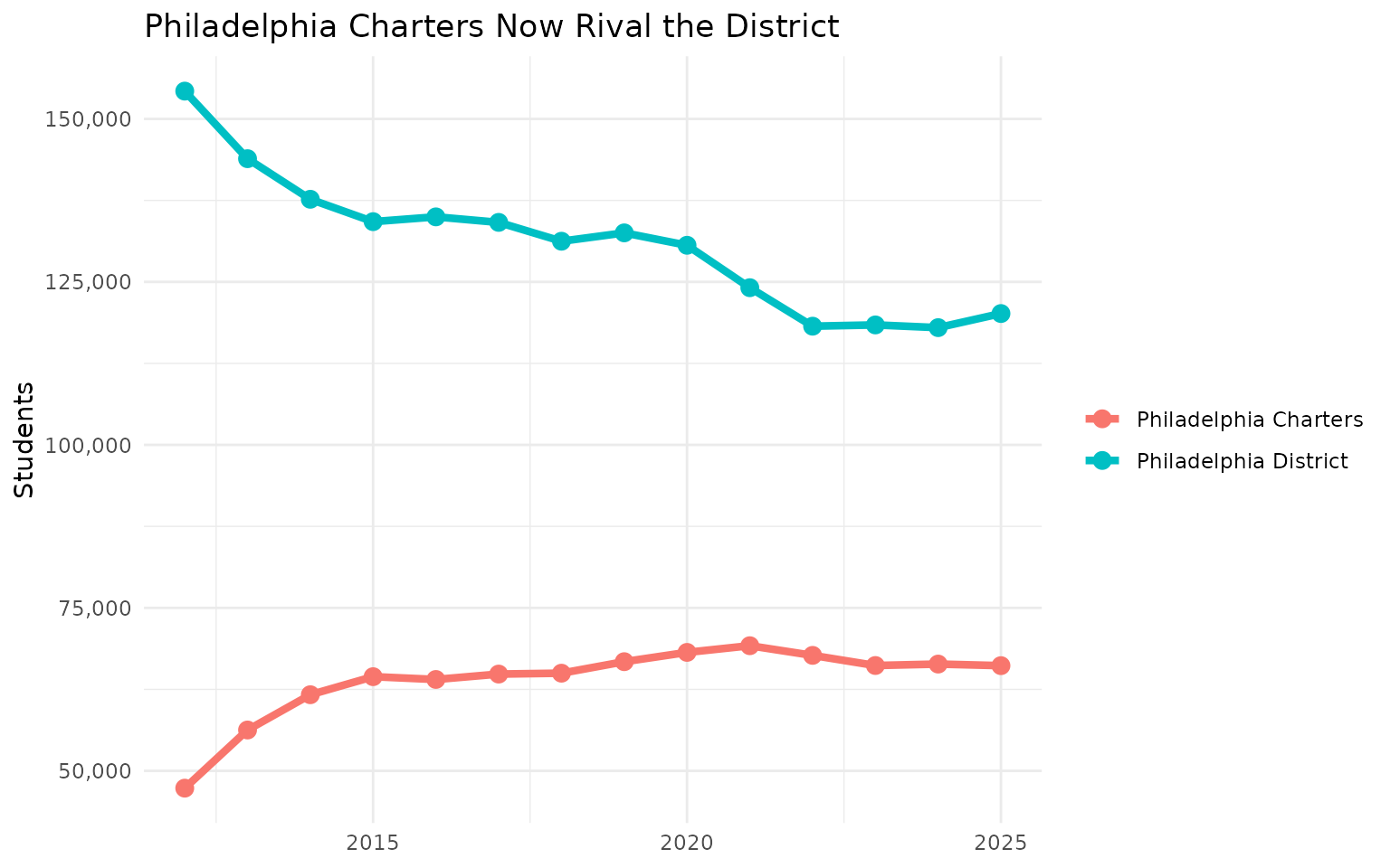
Philadelphia’s charter school sector now enrolls over 60,000 students - more than any single Pennsylvania school district except Philadelphia itself.
15. The great reshuffling: Who won, who lost
reshuffling <- districts %>%
  filter(end_year %in% c(2012, 2024)) %>%
  mutate(category = case_when(
    lea_type == "Cyber CS" ~ "Cyber Charters",
    lea_type == "CS" ~ "Brick-and-Mortar Charters",
    lea_name %in% c("Philadelphia City SD", "Pittsburgh SD") ~ "Big Two Cities",
    county %in% c("Northampton", "Lehigh") ~ "Lehigh Valley",
    county %in% c("Dauphin", "Cumberland", "Lancaster") ~ "Central PA Growth",
    lea_type == "SD" & students < 2000 ~ "Small Rural Districts",
    TRUE ~ "Other Districts"
  )) %>%
  group_by(category, end_year) %>%
  summarize(students = sum(students, na.rm = TRUE), .groups = "drop") %>%
  pivot_wider(names_from = end_year, values_from = students, names_prefix = "y") %>%
  mutate(change = y2024 - y2012)
stopifnot(nrow(reshuffling) > 0)
reshuffling %>% select(category, y2012, y2024, change) %>% arrange(desc(change))
#> # A tibble: 7 × 4
#>   category                    y2012  y2024 change
#>   <chr>                       <dbl>  <dbl>  <dbl>
#> 1 Small Rural Districts      270558 282520  11962
#> 2 Central PA Growth          135050 135818    768
#> 3 Brick-and-Mortar Charters  105036 104277   -759
#> 4 Lehigh Valley               98853  94214  -4639
#> 5 Big Two Cities             180915 137759 -43156
#> 6 Other Districts           1017410 928318 -89092
#> 7 Cyber Charters                 NA  59913     NA

ggplot(reshuffling, aes(x = reorder(category, change), y = change / 1000,
                        fill = change > 0)) +
  geom_col() +
  coord_flip() +
  scale_fill_manual(values = c("#e63946", "#2a9d8f"), guide = "none") +
  labs(title = "The Great Reshuffling: Who Won, Who Lost",
       x = NULL, y = "Change (thousands)") +
  theme_minimal()
#> Warning: Removed 1 row containing missing values or values outside the scale range
#> (`geom_col()`).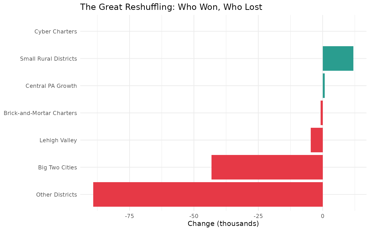
From 2012 to 2024, Pennsylvania lost 65,000 public school students. But the story isn’t uniform decline - it’s a massive reshuffling. Cyber charters and Central PA suburbs gained while the Big Two cities, small rural districts, and other categories lost. The chart above shows the winners and losers.
Session Info
sessionInfo()
#> R version 4.5.2 (2025-10-31)
#> Platform: x86_64-pc-linux-gnu
#> Running under: Ubuntu 24.04.3 LTS
#>
#> Matrix products: default
#> BLAS:   /usr/lib/x86_64-linux-gnu/openblas-pthread/libblas.so.3
#> LAPACK: /usr/lib/x86_64-linux-gnu/openblas-pthread/libopenblasp-r0.3.26.so;  LAPACK version 3.12.0
#>
#> locale:
#>  [1] LC_CTYPE=C.UTF-8       LC_NUMERIC=C           LC_TIME=C.UTF-8
#>  [4] LC_COLLATE=C.UTF-8     LC_MONETARY=C.UTF-8    LC_MESSAGES=C.UTF-8
#>  [7] LC_PAPER=C.UTF-8       LC_NAME=C              LC_ADDRESS=C
#> [10] LC_TELEPHONE=C         LC_MEASUREMENT=C.UTF-8 LC_IDENTIFICATION=C
#>
#> time zone: UTC
#> tzcode source: system (glibc)
#>
#> attached base packages:
#> [1] stats     graphics  grDevices utils     datasets  methods   base
#>
#> other attached packages:
#> [1] ggplot2_4.0.2      tidyr_1.3.2        dplyr_1.2.0        paschooldata_0.1.0
#> [5] testthat_3.3.2
#>
#> loaded via a namespace (and not attached):
#>  [1] gtable_0.3.6       jsonlite_2.0.0     compiler_4.5.2     brio_1.1.5
#>  [5] tidyselect_1.2.1   stringr_1.6.0      jquerylib_0.1.4    systemfonts_1.3.2
#>  [9] scales_1.4.0       textshaping_1.0.5  readxl_1.4.5       yaml_2.3.12
#> [13] fastmap_1.2.0      R6_2.6.1           labeling_0.4.3     generics_0.1.4
#> [17] knitr_1.51         tibble_3.3.1       desc_1.4.3         downloader_0.4.1
#> [21] RColorBrewer_1.1-3 bslib_0.10.0       pillar_1.11.1      rlang_1.1.7
#> [25] utf8_1.2.6         stringi_1.8.7      cachem_1.1.0       xfun_0.56
#> [29] S7_0.2.1           fs_1.6.7           sass_0.4.10        cli_3.6.5
#> [33] withr_3.0.2        pkgdown_2.2.0      magrittr_2.0.4     digest_0.6.39
#> [37] grid_4.5.2         rappdirs_0.3.4     lifecycle_1.0.5    vctrs_0.7.1
#> [41] evaluate_1.0.5     glue_1.8.0         cellranger_1.1.0   farver_2.1.2
#> [45] codetools_0.2-20   ragg_1.5.1         rmarkdown_2.30     purrr_1.2.1
#> [49] tools_4.5.2        pkgconfig_2.0.3    htmltools_0.5.9