Pennsylvania Assessment Data: PSSA and Keystone Results
Source:vignettes/pennsylvania-assessment.Rmd
pennsylvania-assessment.RmdPennsylvania administers two major assessment programs through the Department of Education:
- PSSA (Pennsylvania System of School Assessment): Grades 3-8, testing English Language Arts and Mathematics
- Keystone Exams: End-of-course assessments for grade 11 in Algebra I, Biology, and Literature
This vignette explores assessment data using the
paschooldata package, which provides direct access to PDE’s
assessment files.
Data Notes
PSSA: - Grades 3-8 - Subjects: English Language Arts, Math - Years available: 2015-2019, 2021-2025 (2020 cancelled due to COVID) - Levels: School, District, State
Keystone Exams: - Grade 11 (end-of-course) - Subjects: Algebra I, Biology, Literature - Years available: 2015-2019, 2021-2025
Proficiency Levels: - Below Basic: Limited knowledge - Basic: Partial knowledge - Proficient: Meets grade-level standards - Advanced: Exceeds grade-level standards
Data Source: PA DOE Assessment Data
Data Preparation
# Fetch 2025 assessment data using package functions
pssa_state <- fetch_pssa(2025, level = "state", tidy = FALSE, use_cache = TRUE)
pssa_school <- fetch_pssa(2025, level = "school", tidy = FALSE, use_cache = TRUE)
keystone_state <- fetch_keystone(2025, level = "state", tidy = FALSE, use_cache = TRUE)

# Clean up school data to standard columns
pssa_school <- pssa_school %>%
  select(any_of(c("aun", "county", "district_name", "school_name", "subject",
                  "group", "grade", "n_scored", "pct_advanced", "pct_proficient",
                  "pct_basic", "pct_below_basic", "pct_proficient_above", "end_year")))
1. Only 42% of Pennsylvania students are proficient in math
Less than half of Pennsylvania students meet grade-level math standards. Over 700,000 students took the PSSA Math exam in 2025, and 58% scored below proficient.
state_math <- pssa_state %>%
  filter(subject == "Math",
         group == "All Students",
         grade == "Total") %>%
  select(n_scored, pct_advanced, pct_proficient, pct_basic,
         pct_below_basic, pct_proficient_above)
stopifnot(nrow(state_math) > 0)
state_math
#> # A tibble: 1 × 6
#>   n_scored pct_advanced pct_proficient pct_basic pct_below_basic
#>      <int>        <dbl>          <dbl>     <dbl>           <dbl>
#> 1   703819         16.6           25.1      27.4            30.9
#> # ℹ 1 more variable: pct_proficient_above <dbl>
math_dist <- pssa_state %>%
  filter(subject == "Math",
         group == "All Students",
         grade == "Total") %>%
  select(pct_advanced, pct_proficient, pct_basic, pct_below_basic) %>%
  pivot_longer(everything(), names_to = "Level", values_to = "Percent") %>%
  mutate(Level = gsub("pct_", "", Level),
         Level = tools::toTitleCase(gsub("_", " ", Level)),
         Level = factor(Level, levels = c("Below Basic", "Basic", "Proficient", "Advanced")))
stopifnot(nrow(math_dist) > 0)

ggplot(math_dist, aes(x = Level, y = Percent, fill = Level)) +
  geom_col() +
  scale_fill_manual(values = c("Below Basic" = "#d73027", "Basic" = "#fc8d59",
                                "Proficient" = "#91bfdb", "Advanced" = "#4575b4")) +
  labs(title = "Pennsylvania Math Proficiency Distribution (2025)",
       subtitle = "703,819 students tested",
       x = NULL, y = "Percent of Students") +
  theme_minimal() +
  theme(legend.position = "none")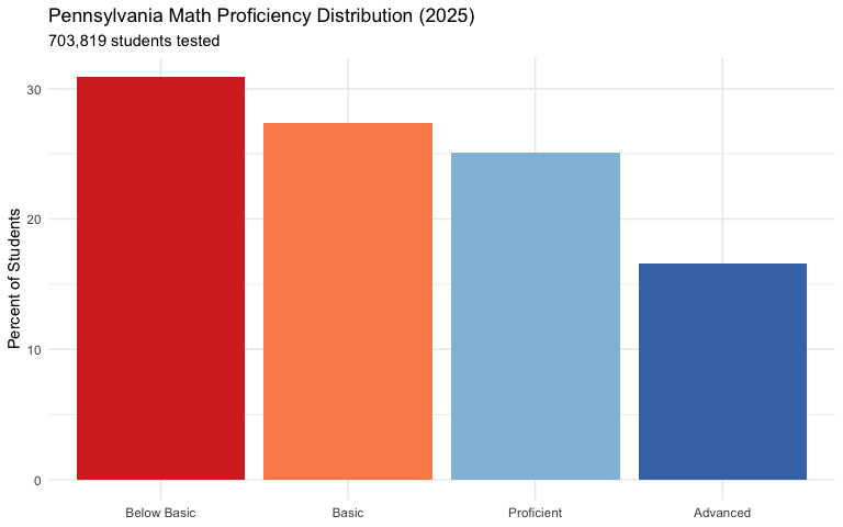
2. ELA outperforms math by 7 percentage points
Nearly half of students (48.5%) meet ELA standards, compared to only 42% in math. The reading-math gap is consistent across grades and persists year over year.
state_ela <- pssa_state %>%
  filter(subject == "English Language Arts",
         group == "All Students",
         grade == "Total") %>%
  select(n_scored, pct_advanced, pct_proficient, pct_basic,
         pct_below_basic, pct_proficient_above)
stopifnot(nrow(state_ela) > 0)
state_ela
#> # A tibble: 1 × 6
#>   n_scored pct_advanced pct_proficient pct_basic pct_below_basic
#>      <int>        <dbl>          <dbl>     <dbl>           <dbl>
#> 1   703650         12.5             36      36.4            15.1
#> # ℹ 1 more variable: pct_proficient_above <dbl>
subjects <- pssa_state %>%
  filter(group == "All Students", grade == "Total") %>%
  select(subject, pct_proficient_above)
stopifnot(nrow(subjects) > 0)

ggplot(subjects, aes(x = subject, y = pct_proficient_above, fill = subject)) +
  geom_col() +
  geom_text(aes(label = paste0(pct_proficient_above, "%")), vjust = -0.5, size = 5) +
  scale_fill_manual(values = c("English Language Arts" = "#4575b4", "Math" = "#d73027")) +
  scale_y_continuous(limits = c(0, 60)) +
  labs(title = "ELA Outperforms Math by 7 Percentage Points",
       subtitle = "2025 PSSA % Proficient and Above",
       x = NULL, y = "% Proficient") +
  theme_minimal() +
  theme(legend.position = "none")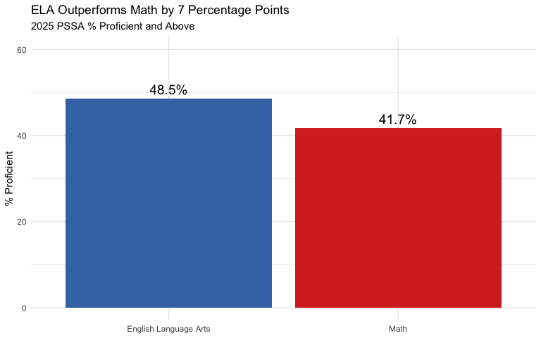
3. Math proficiency drops 23 points from grade 3 to grade 8
Third graders start at 54% proficient in math. By eighth grade, only 31% remain proficient - a 23 percentage point collapse that signals deepening gaps as content becomes more complex.
grade_math <- pssa_state %>%
  filter(subject == "Math",
         group == "All Students",
         grade %in% c("3", "4", "5", "6", "7", "8")) %>%
  select(grade, n_scored, pct_proficient_above) %>%
  arrange(as.numeric(grade))
stopifnot(nrow(grade_math) > 0)
grade_math
#> # A tibble: 6 × 3
#>   grade n_scored pct_proficient_above
#>   <chr>    <int>                <dbl>
#> 1 3       118946                 53.6
#> 2 4       114405                 50.6
#> 3 5       118011                 43.9
#> 4 6       117605                 37.8
#> 5 7       117200                 33.7
#> 6 8       117652                 30.5
grade_math_chart <- pssa_state %>%
  filter(subject == "Math",
         group == "All Students",
         grade %in% c("3", "4", "5", "6", "7", "8")) %>%
  mutate(grade = factor(grade, levels = c("3", "4", "5", "6", "7", "8")))
stopifnot(nrow(grade_math_chart) > 0)

ggplot(grade_math_chart, aes(x = grade, y = pct_proficient_above)) +
  geom_col(fill = "#e63946") +
  geom_text(aes(label = paste0(pct_proficient_above, "%")), vjust = -0.5) +
  scale_y_continuous(limits = c(0, 60)) +
  labs(title = "Math Proficiency Collapses as Students Age",
       subtitle = "2025 PSSA Math - 23 point drop from Grade 3 to Grade 8",
       x = "Grade", y = "% Proficient") +
  theme_minimal()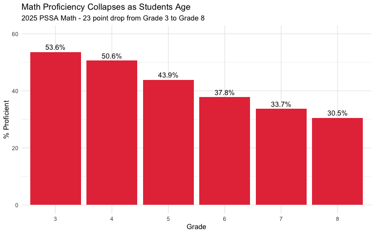
4. Nearly 1 in 3 students score “Below Basic” in math
Almost 28% of Pennsylvania students score at the lowest proficiency level - they haven’t mastered foundational math concepts. This is double the ELA rate.
below_basic <- pssa_state %>%
  filter(group == "All Students", grade == "Total") %>%
  select(subject, pct_below_basic)
stopifnot(nrow(below_basic) > 0)
below_basic
#> # A tibble: 2 × 2
#>   subject               pct_below_basic
#>   <chr>                           <dbl>
#> 1 English Language Arts            15.1
#> 2 Math                             30.9
below_basic_chart <- pssa_state %>%
  filter(group == "All Students", grade == "Total")
stopifnot(nrow(below_basic_chart) > 0)

ggplot(below_basic_chart, aes(x = subject, y = pct_below_basic, fill = subject)) +
  geom_col() +
  geom_text(aes(label = paste0(pct_below_basic, "%")), vjust = -0.5) +
  scale_fill_manual(values = c("English Language Arts" = "#fc8d59", "Math" = "#d73027")) +
  scale_y_continuous(limits = c(0, 35)) +
  labs(title = "Math Has Double the 'Below Basic' Rate of ELA",
       subtitle = "2025 PSSA",
       x = NULL, y = "% Below Basic") +
  theme_minimal() +
  theme(legend.position = "none")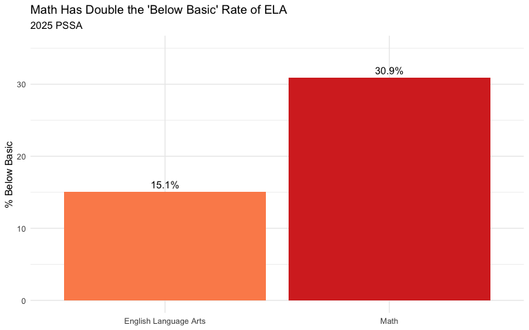
5. Philadelphia’s math proficiency is only 22% - half the state average
Philadelphia City SD’s 170 schools average just 22% math proficiency, compared to 42% statewide. The state’s largest district educates 45,000 tested students but lags dramatically behind.
philly_sum <- pssa_school %>%
  filter(district_name == "PHILADELPHIA CITY SD",
         subject == "Math",
         group == "All Students",
         grade == "Total") %>%
  summarize(
    n_schools = n(),
    total_scored = sum(n_scored, na.rm = TRUE),
    avg_proficient = round(mean(pct_proficient_above, na.rm = TRUE), 1)
  )
stopifnot(nrow(philly_sum) > 0)
philly_sum
#> # A tibble: 1 × 3
#>   n_schools total_scored avg_proficient
#>       <int>        <int>          <dbl>
#> 1       170        45030           21.6
philly_math <- pssa_school %>%
  filter(district_name == "PHILADELPHIA CITY SD",
         subject == "Math",
         group == "All Students",
         grade == "Total") %>%
  filter(!is.na(pct_proficient_above))
stopifnot(nrow(philly_math) > 0)

ggplot(philly_math, aes(x = pct_proficient_above)) +
  geom_histogram(binwidth = 5, fill = "#e63946", color = "white") +
  geom_vline(xintercept = 41.7, linetype = "dashed", color = "#003366", linewidth = 1) +
  annotate("text", x = 50, y = 22, label = "State Avg: 41.7%", color = "#003366") +
  labs(title = "Philadelphia Schools' Math Proficiency Distribution",
       subtitle = "Most schools fall far below state average",
       x = "% Proficient", y = "Number of Schools") +
  theme_minimal()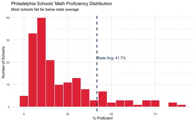
6. Central Bucks outperforms Philadelphia by 45 percentage points
The suburban-urban divide is stark. Central Bucks SD averages 67% math proficiency while Philadelphia averages 22%. Same state assessments, radically different outcomes.
major_districts <- c("PHILADELPHIA CITY SD", "PITTSBURGH SD",
                     "CENTRAL BUCKS SD", "NORTH PENN SD")

dist_compare <- pssa_school %>%
  filter(district_name %in% major_districts,
         subject == "Math",
         group == "All Students",
         grade == "Total") %>%
  group_by(district_name) %>%
  summarize(
    n_schools = n(),
    total_scored = sum(n_scored, na.rm = TRUE),
    avg_proficient = round(mean(pct_proficient_above, na.rm = TRUE), 1),
    .groups = "drop"
  ) %>%
  arrange(desc(avg_proficient))
stopifnot(nrow(dist_compare) > 0)
dist_compare
#> # A tibble: 4 × 4
#>   district_name        n_schools total_scored avg_proficient
#>   <chr>                    <int>        <int>          <dbl>
#> 1 CENTRAL BUCKS SD            20         7684           66.8
#> 2 NORTH PENN SD               16         5361           61.4
#> 3 PITTSBURGH SD               48         7114           26.2
#> 4 PHILADELPHIA CITY SD       170        45030           21.6
district_summary <- pssa_school %>%
  filter(district_name %in% major_districts,
         subject == "Math",
         group == "All Students",
         grade == "Total") %>%
  group_by(district_name) %>%
  summarize(avg_proficient = mean(pct_proficient_above, na.rm = TRUE),
            .groups = "drop")
stopifnot(nrow(district_summary) > 0)

ggplot(district_summary, aes(x = reorder(district_name, avg_proficient),
                              y = avg_proficient,
                              fill = avg_proficient > 40)) +
  geom_col() +
  coord_flip() +
  scale_fill_manual(values = c("TRUE" = "#2a9d8f", "FALSE" = "#e63946")) +
  labs(title = "The Urban-Suburban Divide",
       subtitle = "2025 PSSA Math % Proficient",
       x = NULL, y = "% Proficient") +
  theme_minimal() +
  theme(legend.position = "none")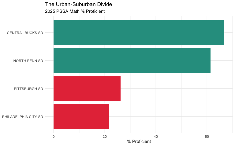
7. Peters Township leads the state at 88% math proficiency
Pennsylvania’s top-performing districts cluster in the Pittsburgh suburbs (Allegheny County) and Philadelphia suburbs (Montgomery, Delaware, Chester counties). The top 10 all exceed 77% proficiency.
top_dist <- pssa_school %>%
  filter(subject == "Math",
         group == "All Students",
         grade == "Total") %>%
  group_by(district_name, county) %>%
  summarize(
    n_schools = n(),
    total_scored = sum(n_scored, na.rm = TRUE),
    avg_proficient = round(mean(pct_proficient_above, na.rm = TRUE), 1),
    .groups = "drop"
  ) %>%
  filter(total_scored >= 500) %>%
  arrange(desc(avg_proficient)) %>%
  head(10)
stopifnot(nrow(top_dist) > 0)
top_dist
#> # A tibble: 10 × 5
#>    district_name             county     n_schools total_scored avg_proficient
#>    <chr>                     <chr>          <int>        <int>          <dbl>
#>  1 PETERS TOWNSHIP SD        WASHINGTON         4         1784           87.9
#>  2 FOX CHAPEL AREA SD        ALLEGHENY          5         1906           84.3
#>  3 UPPER ST. CLAIR SD        ALLEGHENY          5         1793           84.1
#>  4 LOWER MERION SD           MONTGOMERY         9         3678           82.7
#>  5 HAMPTON TOWNSHIP SD       ALLEGHENY          4         1156           82.4
#>  6 RADNOR TOWNSHIP SD        DELAWARE           4         1575           82.3
#>  7 WEST ALLEGHENY SD         ALLEGHENY          4         1518           82.2
#>  8 COLONIAL SD               MONTGOMERY         6         2526           79.7
#>  9 NORTH ALLEGHENY SD        ALLEGHENY         10         3887           79.4
#> 10 WALLINGFORD-SWARTHMORE SD DELAWARE           4         1706           78.5
top_districts <- pssa_school %>%
  filter(subject == "Math",
         group == "All Students",
         grade == "Total") %>%
  group_by(district_name) %>%
  summarize(
    total_scored = sum(n_scored, na.rm = TRUE),
    avg_proficient = mean(pct_proficient_above, na.rm = TRUE),
    .groups = "drop"
  ) %>%
  filter(total_scored >= 500) %>%
  arrange(desc(avg_proficient)) %>%
  head(10)
stopifnot(nrow(top_districts) > 0)

ggplot(top_districts, aes(x = reorder(district_name, avg_proficient),
                           y = avg_proficient)) +
  geom_col(fill = "#2a9d8f") +
  coord_flip() +
  labs(title = "Pennsylvania's Top 10 Math Districts (2025)",
       subtitle = "Districts with 500+ students tested",
       x = NULL, y = "% Proficient") +
  theme_minimal()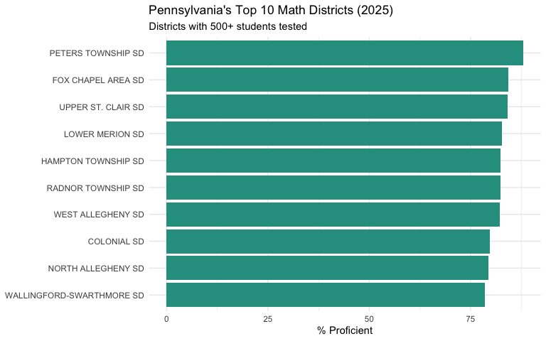
8. Harrisburg has the worst math proficiency of any large district at 6%
Among Pennsylvania’s major urban districts, Harrisburg City SD has the lowest math proficiency at just 5.7%. Even Pittsburgh and Philadelphia outperform the state capital.
urban_districts <- c("PHILADELPHIA CITY SD", "PITTSBURGH SD",
                     "ALLENTOWN CITY SD", "READING SD", "ERIE CITY SD",
                     "SCRANTON SD", "HARRISBURG CITY SD", "LANCASTER SD")

urban_dist <- pssa_school %>%
  filter(district_name %in% urban_districts,
         subject == "Math",
         group == "All Students",
         grade == "Total") %>%
  group_by(district_name) %>%
  summarize(
    n_schools = n(),
    total_scored = sum(n_scored, na.rm = TRUE),
    avg_proficient = round(mean(pct_proficient_above, na.rm = TRUE), 1),
    .groups = "drop"
  ) %>%
  arrange(desc(avg_proficient))
stopifnot(nrow(urban_dist) > 0)
urban_dist
#> # A tibble: 8 × 4
#>   district_name        n_schools total_scored avg_proficient
#>   <chr>                    <int>        <int>          <dbl>
#> 1 SCRANTON SD                 14         3281           27
#> 2 LANCASTER SD                18         3799           26.9
#> 3 PITTSBURGH SD               48         7114           26.2
#> 4 PHILADELPHIA CITY SD       170        45030           21.6
#> 5 ALLENTOWN CITY SD           17         5887           19.3
#> 6 ERIE CITY SD                13         3864           15.1
#> 7 READING SD                  18         6227           14.5
#> 8 HARRISBURG CITY SD          10         2571            5.7
urban_summary <- pssa_school %>%
  filter(district_name %in% urban_districts,
         subject == "Math",
         group == "All Students",
         grade == "Total") %>%
  group_by(district_name) %>%
  summarize(avg_proficient = mean(pct_proficient_above, na.rm = TRUE),
            .groups = "drop")
stopifnot(nrow(urban_summary) > 0)

ggplot(urban_summary, aes(x = reorder(district_name, avg_proficient),
                           y = avg_proficient)) +
  geom_col(fill = "#e63946") +
  geom_hline(yintercept = 41.7, linetype = "dashed", color = "#003366") +
  annotate("text", x = 6, y = 44, label = "State Avg: 41.7%", color = "#003366") +
  coord_flip() +
  labs(title = "Pennsylvania's Big City Math Crisis",
       subtitle = "All major urban districts below state average",
       x = NULL, y = "% Proficient") +
  theme_minimal()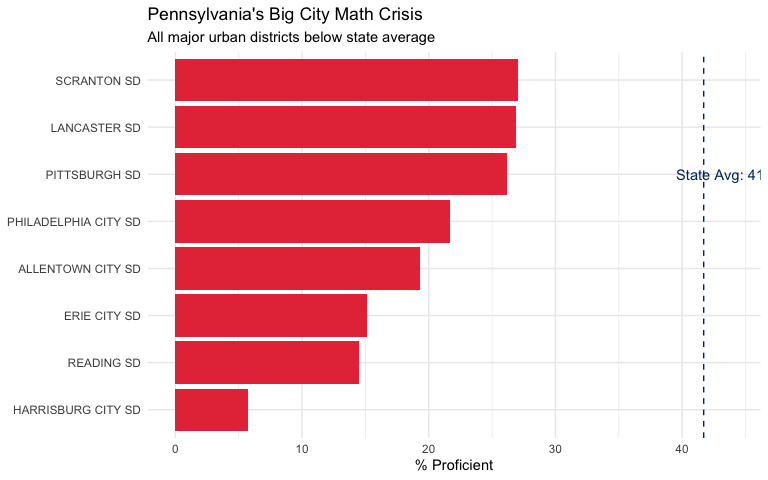
9. Keystone Literature leads at 62% proficiency
Among the three Keystone end-of-course exams, Literature has the highest proficiency at 62%, followed by Biology at 49% and Algebra I trailing at 44%.
keystone_ov <- keystone_state %>%
  filter(group == "All Students") %>%
  select(subject, n_scored, pct_proficient_above) %>%
  arrange(desc(pct_proficient_above))
stopifnot(nrow(keystone_ov) > 0)
keystone_ov
#> # A tibble: 3 × 3
#>   subject    n_scored pct_proficient_above
#>   <chr>         <int>                <dbl>
#> 1 Literature   120804                 62.1
#> 2 Biology      121380                 49.4
#> 3 Algebra I    121876                 44.3
keystone_chart_data <- keystone_state %>%
  filter(group == "All Students")
stopifnot(nrow(keystone_chart_data) > 0)

ggplot(keystone_chart_data, aes(x = reorder(subject, pct_proficient_above),
             y = pct_proficient_above,
             fill = subject)) +
  geom_col() +
  geom_text(aes(label = paste0(pct_proficient_above, "%")), hjust = -0.2) +
  coord_flip() +
  scale_fill_brewer(palette = "Set2") +
  scale_y_continuous(limits = c(0, 80)) +
  labs(title = "Keystone Exam Proficiency Rates (2025)",
       subtitle = "Grade 11 End-of-Course Exams",
       x = NULL, y = "% Proficient") +
  theme_minimal() +
  theme(legend.position = "none")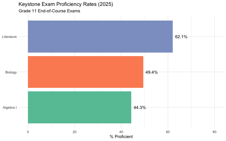
10. Nearly 1 in 5 students score “Below Basic” on Algebra I
Algebra I has the highest failure rate among Keystone exams - 19% score “Below Basic.” These students are graduating high school without basic algebraic understanding.
keystone_bb <- keystone_state %>%
  filter(group == "All Students") %>%
  select(subject, pct_below_basic) %>%
  arrange(desc(pct_below_basic))
stopifnot(nrow(keystone_bb) > 0)
keystone_bb
#> # A tibble: 3 × 2
#>   subject    pct_below_basic
#>   <chr>                <dbl>
#> 1 Biology               23.4
#> 2 Algebra I             19.3
#> 3 Literature            13.7
keystone_long <- keystone_state %>%
  filter(group == "All Students") %>%
  select(subject, pct_advanced, pct_proficient, pct_basic, pct_below_basic) %>%
  pivot_longer(-subject, names_to = "Level", values_to = "Percent") %>%
  mutate(Level = gsub("pct_", "", Level),
         Level = tools::toTitleCase(gsub("_", " ", Level)),
         Level = factor(Level, levels = c("Below Basic", "Basic", "Proficient", "Advanced")))
stopifnot(nrow(keystone_long) > 0)

ggplot(keystone_long, aes(x = subject, y = Percent, fill = Level)) +
  geom_col(position = "stack") +
  scale_fill_manual(values = c("Below Basic" = "#d73027", "Basic" = "#fc8d59",
                                "Proficient" = "#91bfdb", "Advanced" = "#4575b4")) +
  labs(title = "Keystone Proficiency Distribution by Subject",
       subtitle = "2025 Grade 11 Results - 120,000+ students per exam",
       x = NULL, y = "Percent") +
  theme_minimal() +
  theme(legend.position = "bottom")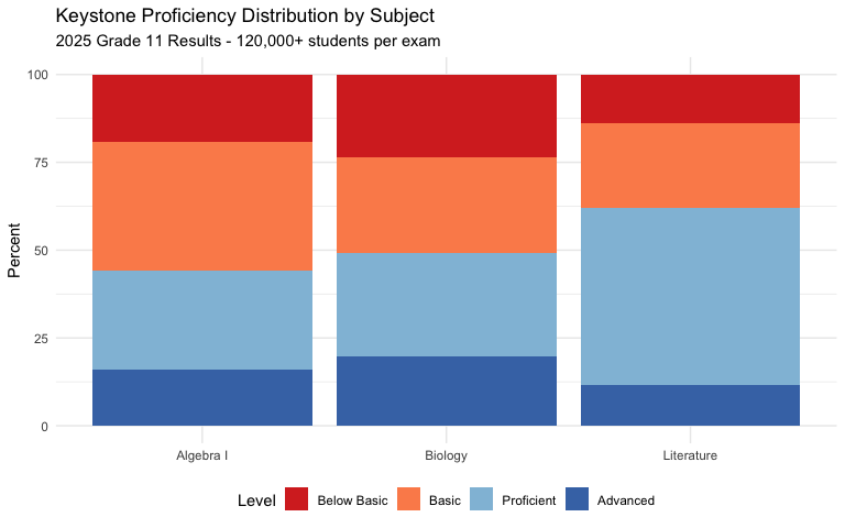
11. Asian students outperform all other groups by 17+ points in math
Asian students lead with 68% math proficiency, followed by White students at 51%. Black and Hispanic students trail at 16% and 22% respectively - a gap of over 50 percentage points.
racial_groups <- c("White (not Hispanic)", "Black or African American (not Hispanic)",
                   "Hispanic (any race)", "Asian (not Hispanic)")

racial_gap <- pssa_state %>%
  filter(subject == "Math",
         group %in% racial_groups,
         grade == "Total") %>%
  select(group, n_scored, pct_proficient_above) %>%
  arrange(desc(pct_proficient_above))
stopifnot(nrow(racial_gap) > 0)
racial_gap
#> # A tibble: 4 × 3
#>   group                                    n_scored pct_proficient_above
#>   <chr>                                       <int>                <dbl>
#> 1 Asian (not Hispanic)                        35601                 68.4
#> 2 White (not Hispanic)                       424531                 50.8
#> 3 Hispanic (any race)                        105681                 21.7
#> 4 Black or African American (not Hispanic)    97352                 15.7
race_data <- pssa_state %>%
  filter(subject == "Math",
         group %in% racial_groups,
         grade == "Total") %>%
  mutate(group = gsub(" \\(not Hispanic\\)", "", group),
         group = gsub(" \\(any race\\)", "", group))
stopifnot(nrow(race_data) > 0)

ggplot(race_data, aes(x = reorder(group, pct_proficient_above),
                       y = pct_proficient_above,
                       fill = group)) +
  geom_col() +
  coord_flip() +
  scale_fill_brewer(palette = "Set2") +
  labs(title = "Racial Achievement Gaps in Math",
       subtitle = "2025 PSSA - 52 point gap between highest and lowest",
       x = NULL, y = "% Proficient") +
  theme_minimal() +
  theme(legend.position = "none")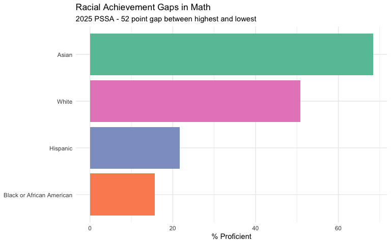
12. Economically disadvantaged students face a 16-point gap
Students from low-income families score 26% proficient in math, compared to the state average of 42%. The poverty gap is larger in ELA (16 points) than math (16 points).
econ_disadv <- pssa_state %>%
  filter(subject == "Math",
         group %in% c("All Students", "Economically Disadvantaged"),
         grade == "Total") %>%
  select(group, n_scored, pct_proficient_above)
stopifnot(nrow(econ_disadv) > 0)
econ_disadv
#> # A tibble: 2 × 3
#>   group                      n_scored pct_proficient_above
#>   <chr>                         <int>                <dbl>
#> 1 All Students                 703819                 41.7
#> 2 Economically Disadvantaged   338533                 25.5
econ_gap_data <- pssa_state %>%
  filter(group %in% c("All Students", "Economically Disadvantaged"),
         grade == "Total")
stopifnot(nrow(econ_gap_data) > 0)

ggplot(econ_gap_data, aes(x = subject, y = pct_proficient_above, fill = group)) +
  geom_col(position = "dodge") +
  geom_text(aes(label = paste0(pct_proficient_above, "%")),
            position = position_dodge(width = 0.9), vjust = -0.5) +
  scale_fill_manual(values = c("All Students" = "#003366",
                                "Economically Disadvantaged" = "#e63946"),
                    name = "Group") +
  scale_y_continuous(limits = c(0, 60)) +
  labs(title = "The Income Achievement Gap",
       subtitle = "2025 PSSA - 16 point gap in both subjects",
       x = NULL, y = "% Proficient") +
  theme_minimal() +
  theme(legend.position = "bottom")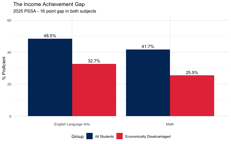
13. IEP students have the lowest proficiency rates at 15%
Students with Individualized Education Programs (IEPs) score just 15% proficient in math and 17% in ELA. English Language Learners (ELL) score similarly low at 14% in ELA and 16% in math.
iep_compare <- pssa_state %>%
  filter(group %in% c("All Students", "IEP", "ELL", "Economically Disadvantaged"),
         grade == "Total") %>%
  select(subject, group, n_scored, pct_proficient_above) %>%
  arrange(subject, desc(pct_proficient_above))
stopifnot(nrow(iep_compare) > 0)
iep_compare
#> # A tibble: 8 × 4
#>   subject               group                      n_scored pct_proficient_above
#>   <chr>                 <chr>                         <int>                <dbl>
#> 1 English Language Arts All Students                 703650                 48.5
#> 2 English Language Arts Economically Disadvantaged   338525                 32.7
#> 3 English Language Arts IEP                          143647                 16.5
#> 4 English Language Arts ELL                           41754                 13.8
#> 5 Math                  All Students                 703819                 41.7
#> 6 Math                  Economically Disadvantaged   338533                 25.5
#> 7 Math                  ELL                           41980                 16
#> 8 Math                  IEP                          143413                 15.3
subgroups <- pssa_state %>%
  filter(subject == "Math",
         group %in% c("All Students", "IEP", "ELL", "Economically Disadvantaged"),
         grade == "Total")
stopifnot(nrow(subgroups) > 0)

ggplot(subgroups, aes(x = reorder(group, pct_proficient_above),
                       y = pct_proficient_above,
                       fill = group == "All Students")) +
  geom_col() +
  coord_flip() +
  scale_fill_manual(values = c("TRUE" = "#003366", "FALSE" = "#e63946")) +
  labs(title = "Achievement Gaps Across Student Subgroups",
       subtitle = "2025 PSSA Math - All subgroups below state average",
       x = NULL, y = "% Proficient") +
  theme_minimal() +
  theme(legend.position = "none")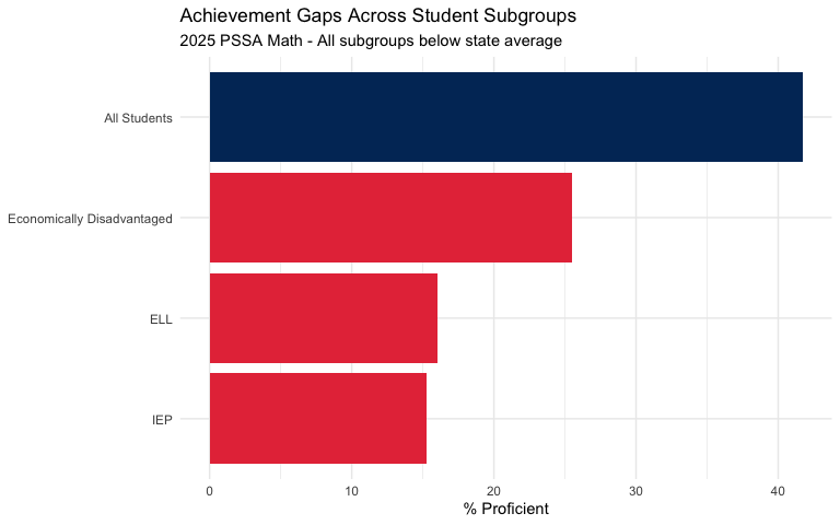
14. Female students outperform males in ELA by 9 points
Girls score 53% proficient in ELA compared to 44% for boys - a 9 percentage point gap. But boys slightly outperform girls in math (43% vs 40%).
gender_gap <- pssa_state %>%
  filter(group %in% c("Male", "Female"),
         grade == "Total") %>%
  select(subject, group, n_scored, pct_proficient_above) %>%
  arrange(subject, desc(pct_proficient_above))
stopifnot(nrow(gender_gap) > 0)
gender_gap
#> # A tibble: 4 × 4
#>   subject               group  n_scored pct_proficient_above
#>   <chr>                 <chr>     <int>                <dbl>
#> 1 English Language Arts Female   344499                 52.9
#> 2 English Language Arts Male     359151                 44.2
#> 3 Math                  Male     359347                 43.1
#> 4 Math                  Female   344472                 40.2
gender_data <- pssa_state %>%
  filter(group %in% c("Male", "Female"),
         grade == "Total")
stopifnot(nrow(gender_data) > 0)

ggplot(gender_data, aes(x = subject, y = pct_proficient_above, fill = group)) +
  geom_col(position = "dodge") +
  geom_text(aes(label = paste0(pct_proficient_above, "%")),
            position = position_dodge(width = 0.9), vjust = -0.5) +
  scale_fill_manual(values = c("Female" = "#e377c2", "Male" = "#1f77b4")) +
  scale_y_continuous(limits = c(0, 65)) +
  labs(title = "Gender Gaps in PSSA Performance",
       subtitle = "2025 Results - Girls lead ELA, boys edge ahead in math",
       x = NULL, y = "% Proficient") +
  theme_minimal() +
  theme(legend.position = "bottom")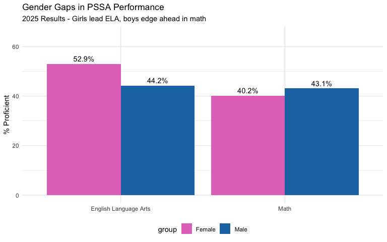
15. The “Advanced” category is shrinking - only 17% in math
Only 17% of students score “Advanced” in math, while 13% reach Advanced in ELA. The top tier is thin, with most proficient students clustered in the “Proficient” category rather than excelling.
adv_rates <- pssa_state %>%
  filter(group == "All Students",
         grade == "Total") %>%
  select(subject, pct_advanced, pct_proficient)
stopifnot(nrow(adv_rates) > 0)
adv_rates
#> # A tibble: 2 × 3
#>   subject               pct_advanced pct_proficient
#>   <chr>                        <dbl>          <dbl>
#> 1 English Language Arts         12.5           36
#> 2 Math                          16.6           25.1
advanced_by_grade <- pssa_state %>%
  filter(subject == "Math",
         group == "All Students",
         grade %in% c("3", "4", "5", "6", "7", "8")) %>%
  mutate(grade = factor(grade, levels = c("3", "4", "5", "6", "7", "8")))
stopifnot(nrow(advanced_by_grade) > 0)

ggplot(advanced_by_grade, aes(x = grade, y = pct_advanced)) +
  geom_col(fill = "#4575b4") +
  geom_text(aes(label = paste0(pct_advanced, "%")), vjust = -0.5) +
  scale_y_continuous(limits = c(0, 30)) +
  labs(title = "Where Are the Advanced Math Students?",
       subtitle = "2025 PSSA % Advanced by Grade - Peaks at grade 3, drops steadily",
       x = "Grade", y = "% Advanced") +
  theme_minimal()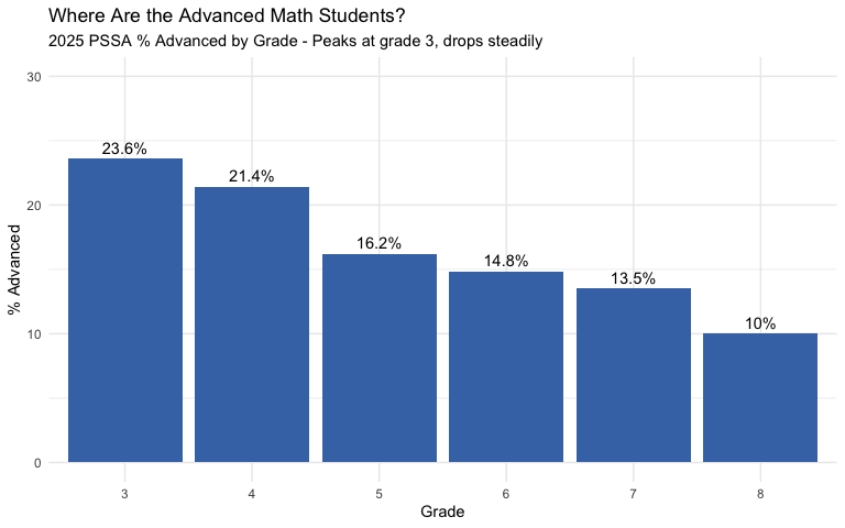
16. Chester Community CS has the lowest math proficiency at 4%
Among schools with substantial enrollment (300+ students tested), Chester Community Charter School has just 3.7% math proficiency - the lowest in Pennsylvania.
bottom_dist <- pssa_school %>%
  filter(subject == "Math",
         group == "All Students",
         grade == "Total") %>%
  group_by(district_name, county) %>%
  summarize(
    n_schools = n(),
    total_scored = sum(n_scored, na.rm = TRUE),
    avg_proficient = round(mean(pct_proficient_above, na.rm = TRUE), 1),
    .groups = "drop"
  ) %>%
  filter(total_scored >= 300) %>%
  arrange(avg_proficient) %>%
  head(10)
stopifnot(nrow(bottom_dist) > 0)
bottom_dist
#> # A tibble: 10 × 5
#>    district_name                    county n_schools total_scored avg_proficient
#>    <chr>                            <chr>      <int>        <int>          <dbl>
#>  1 CHESTER COMMUNITY CS             DELAW…         1         2282            3.7
#>  2 LINDLEY ACADEMY CS AT BIRNEY     PHILA…         1          438            4.1
#>  3 GREATER JOHNSTOWN SD             CAMBR…         4         1022            4.3
#>  4 KIPP NORTH PHILADELPHIA CS       PHILA…         1          338            4.4
#>  5 MEMPHIS STREET ACADEMY CS @ JP … PHILA…         1          420            4.5
#>  6 ALLIANCE FOR PROGRESS CS         PHILA…         1          379            4.7
#>  7 ALIQUIPPA SD                     BEAVER         2          392            5
#>  8 ESPERANZA ACADEMY CS             PHILA…         1          716            5.2
#>  9 INSIGHT PA CYBER CS              CHEST…         1          989            5.4
#> 10 HARRISBURG CITY SD               DAUPH…        10         2571            5.7
bottom_districts <- pssa_school %>%
  filter(subject == "Math",
         group == "All Students",
         grade == "Total") %>%
  group_by(district_name) %>%
  summarize(
    total_scored = sum(n_scored, na.rm = TRUE),
    avg_proficient = mean(pct_proficient_above, na.rm = TRUE),
    .groups = "drop"
  ) %>%
  filter(total_scored >= 300) %>%
  arrange(avg_proficient) %>%
  head(10)
stopifnot(nrow(bottom_districts) > 0)

ggplot(bottom_districts, aes(x = reorder(district_name, -avg_proficient),
                              y = avg_proficient)) +
  geom_col(fill = "#d73027") +
  coord_flip() +
  labs(title = "Pennsylvania's Lowest-Performing Districts (2025)",
       subtitle = "Districts with 300+ students tested",
       x = NULL, y = "% Proficient") +
  theme_minimal()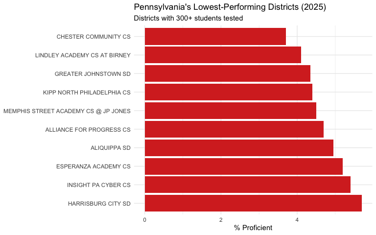
17. Third grade reading is the gateway - 49% are already behind
Only 49% of third graders are proficient in ELA. Since third grade is when students transition from “learning to read” to “reading to learn,” half of Pennsylvania’s students start behind in every subject.
grade3_ela <- pssa_state %>%
  filter(subject == "English Language Arts",
         group == "All Students",
         grade %in% c("3", "4", "5", "6", "7", "8")) %>%
  select(grade, n_scored, pct_proficient_above) %>%
  arrange(as.numeric(grade))
stopifnot(nrow(grade3_ela) > 0)
grade3_ela
#> # A tibble: 6 × 3
#>   grade n_scored pct_proficient_above
#>   <chr>    <int>                <dbl>
#> 1 3       118825                 48.6
#> 2 4       114210                 48.4
#> 3 5       117850                 44.7
#> 4 6       117599                 50.8
#> 5 7       117288                 49.2
#> 6 8       117878                 49.3
ela_by_grade <- pssa_state %>%
  filter(subject == "English Language Arts",
         group == "All Students",
         grade %in% c("3", "4", "5", "6", "7", "8")) %>%
  mutate(grade = factor(grade, levels = c("3", "4", "5", "6", "7", "8")))
stopifnot(nrow(ela_by_grade) > 0)

ggplot(ela_by_grade, aes(x = grade, y = pct_proficient_above)) +
  geom_col(fill = "#003366") +
  geom_hline(yintercept = 50, linetype = "dashed", color = "#e63946") +
  annotate("text", x = 5.5, y = 52, label = "50% threshold", color = "#e63946") +
  labs(title = "ELA Proficiency by Grade",
       subtitle = "2025 PSSA - Nearly half start below proficient at grade 3",
       x = "Grade", y = "% Proficient") +
  theme_minimal()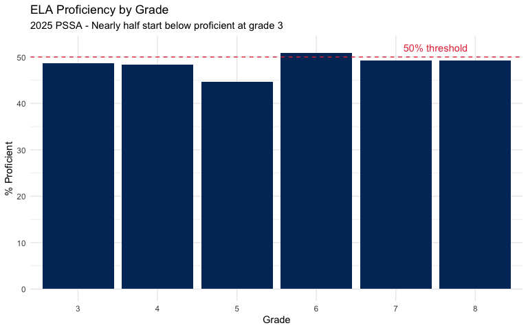
Session Info
sessionInfo()
#> R version 4.5.2 (2025-10-31)
#> Platform: x86_64-pc-linux-gnu
#> Running under: Ubuntu 24.04.3 LTS
#>
#> Matrix products: default
#> BLAS:   /usr/lib/x86_64-linux-gnu/openblas-pthread/libblas.so.3
#> LAPACK: /usr/lib/x86_64-linux-gnu/openblas-pthread/libopenblasp-r0.3.26.so;  LAPACK version 3.12.0
#>
#> locale:
#>  [1] LC_CTYPE=C.UTF-8       LC_NUMERIC=C           LC_TIME=C.UTF-8
#>  [4] LC_COLLATE=C.UTF-8     LC_MONETARY=C.UTF-8    LC_MESSAGES=C.UTF-8
#>  [7] LC_PAPER=C.UTF-8       LC_NAME=C              LC_ADDRESS=C
#> [10] LC_TELEPHONE=C         LC_MEASUREMENT=C.UTF-8 LC_IDENTIFICATION=C
#>
#> time zone: UTC
#> tzcode source: system (glibc)
#>
#> attached base packages:
#> [1] stats     graphics  grDevices utils     datasets  methods   base
#>
#> other attached packages:
#> [1] readxl_1.4.5       ggplot2_4.0.2      tidyr_1.3.2        dplyr_1.2.0
#> [5] paschooldata_0.1.0
#>
#> loaded via a namespace (and not attached):
#>  [1] gtable_0.3.6       jsonlite_2.0.0     compiler_4.5.2     tidyselect_1.2.1
#>  [5] jquerylib_0.1.4    systemfonts_1.3.2  scales_1.4.0       textshaping_1.0.5
#>  [9] yaml_2.3.12        fastmap_1.2.0      R6_2.6.1           labeling_0.4.3
#> [13] generics_0.1.4     knitr_1.51         tibble_3.3.1       desc_1.4.3
#> [17] downloader_0.4.1   bslib_0.10.0       pillar_1.11.1      RColorBrewer_1.1-3
#> [21] rlang_1.1.7        utf8_1.2.6         cachem_1.1.0       xfun_0.56
#> [25] S7_0.2.1           fs_1.6.7           sass_0.4.10        cli_3.6.5
#> [29] withr_3.0.2        pkgdown_2.2.0      magrittr_2.0.4     digest_0.6.39
#> [33] grid_4.5.2         rappdirs_0.3.4     lifecycle_1.0.5    vctrs_0.7.1
#> [37] evaluate_1.0.5     glue_1.8.0         cellranger_1.1.0   farver_2.1.2
#> [41] codetools_0.2-20   ragg_1.5.1         rmarkdown_2.30     purrr_1.2.1
#> [45] tools_4.5.2        pkgconfig_2.0.3    htmltools_0.5.9