West Virginia educates roughly 250,000 students across 55 county school districts – one for each county. From the coalfields of McDowell to the Eastern Panhandle suburbs of DC, here are fifteen stories hiding in the data.
Part of the njschooldata family.
Full documentation — all 15 stories with interactive charts, getting-started guide, and complete function reference.
Highlights
library(wvschooldata)
library(dplyr)
library(tidyr)
library(ggplot2)

theme_set(theme_minimal(base_size = 14))

enr_2024 <- fetch_enr(2024, use_cache = TRUE)
1. Coal country has the smallest districts
The southern coalfield counties – McDowell, Wyoming, Mingo, Logan, and Boone – have experienced decades of population loss as the coal industry contracted.
# Coal counties
coal_counties <- c("MCDOWELL", "WYOMING", "MINGO", "LOGAN", "BOONE")

coal_districts <- enr_2024 |>
  filter(is_district, county %in% coal_counties,
         subgroup == "total_enrollment", grade_level == "TOTAL") |>
  select(district_name, county, n_students) |>
  arrange(n_students)

coal_districts
#> # A tibble: 5 x 3
#> district_name county n_students
#> <chr> <chr> <dbl>
#> 1 MCDOWELL COUNTY SCHOOLS MCDOWELL 2393
#> 2 WYOMING COUNTY SCHOOLS WYOMING 3172
#> 3 BOONE COUNTY SCHOOLS BOONE 3100
#> 4 MINGO COUNTY SCHOOLS MINGO 3573
#> 5 LOGAN COUNTY SCHOOLS LOGAN 4771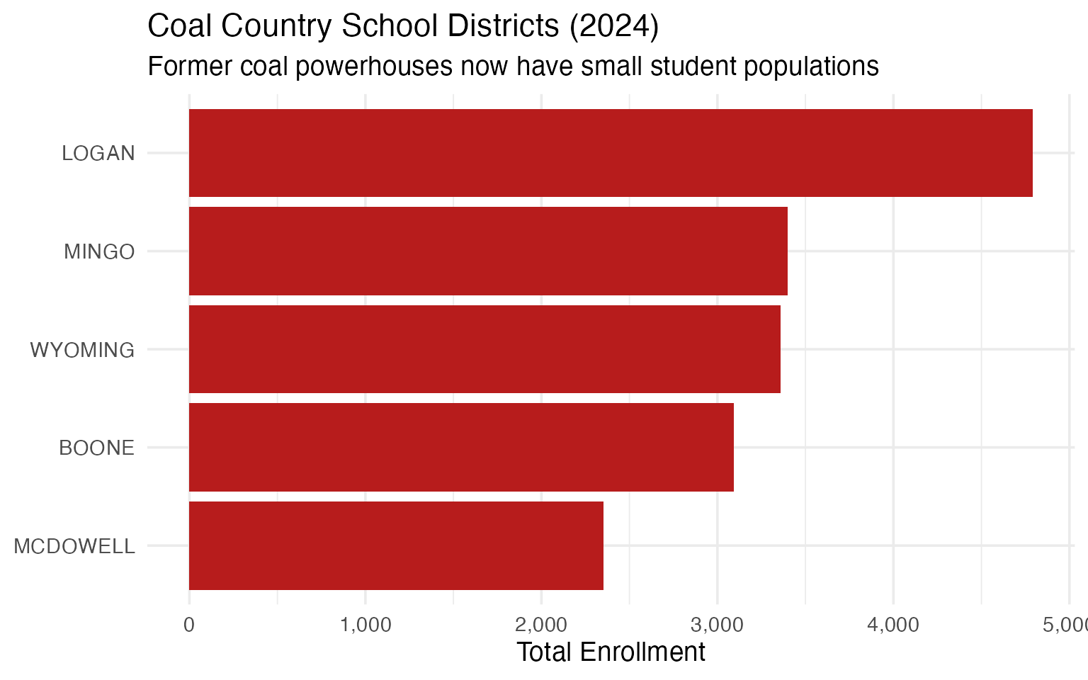
2. The Eastern Panhandle has the largest suburban districts
The Eastern Panhandle – Berkeley, Jefferson, and Morgan counties near Washington, D.C. – benefits from suburban spillover and has some of the state’s fastest-growing areas.
# Eastern Panhandle counties (DC suburbs)
panhandle <- c("BERKELEY", "JEFFERSON", "MORGAN")

regional_comparison <- enr_2024 |>
  filter(is_district, subgroup == "total_enrollment", grade_level == "TOTAL") |>
  mutate(region = case_when(
    county %in% panhandle ~ "Eastern Panhandle",
    TRUE ~ "Rest of State"
  )) |>
  group_by(region) |>
  summarize(
    n_districts = n(),
    total_students = sum(n_students, na.rm = TRUE),
    avg_district_size = round(mean(n_students), 0),
    .groups = "drop"
  )

regional_comparison
#> # A tibble: 2 x 4
#> region n_districts total_students avg_district_size
#> <chr> <int> <dbl> <dbl>
#> 1 Eastern Panhandle 3 30173 10058
#> 2 Rest of State 52 212604 4088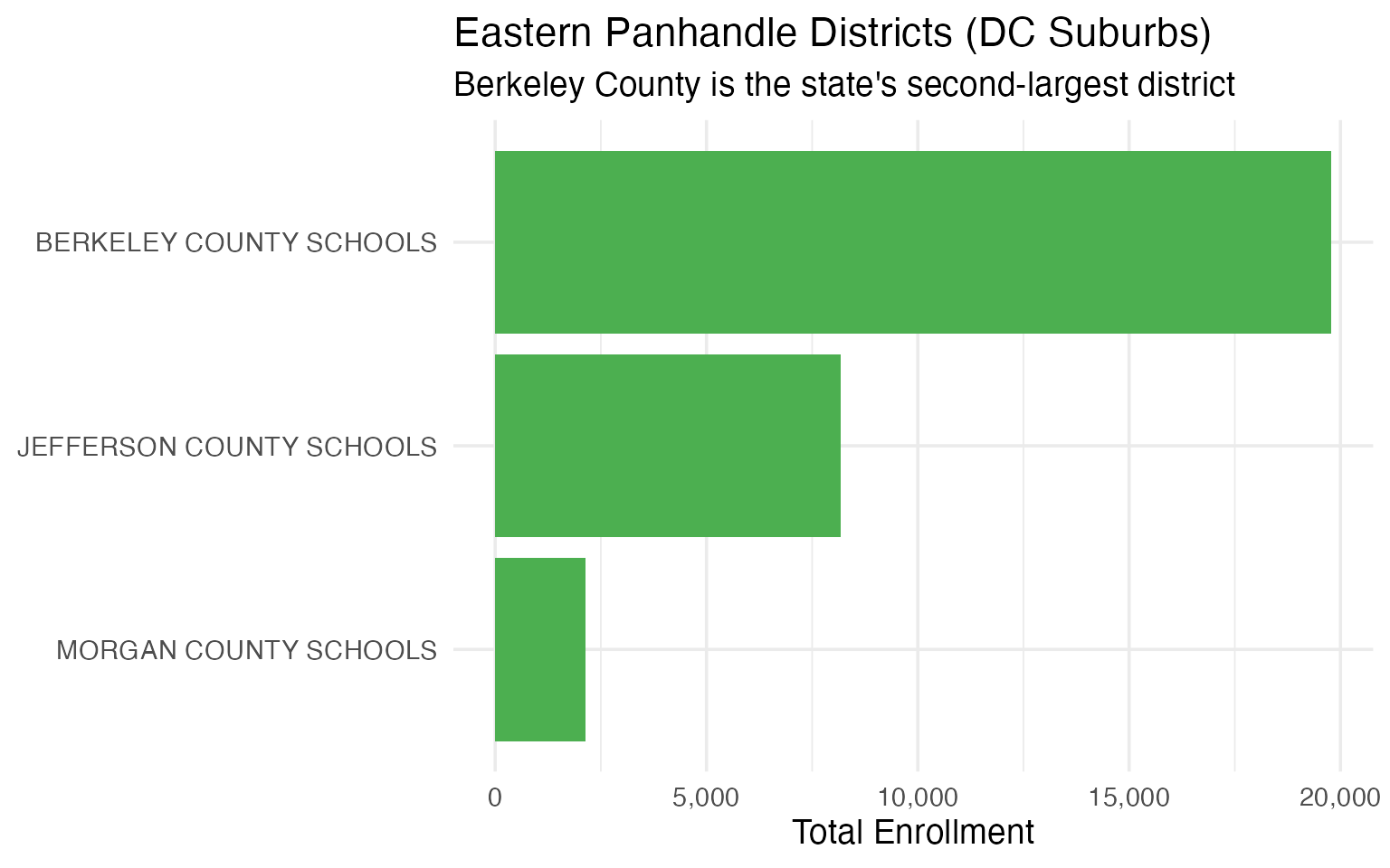
3. The urban-rural divide is minimal
West Virginia has no large cities. Even “urban” Kanawha County is mostly rural by national standards. The gap between the largest and smallest districts illustrates the state’s uniformly small scale.
district_sizes <- enr_2024 |>
  filter(is_district, subgroup == "total_enrollment", grade_level == "TOTAL") |>
  arrange(desc(n_students)) |>
  mutate(rank = row_number()) |>
  select(rank, district_name, county, n_students)

size_range <- tibble(
  metric = c("Largest (Kanawha)", "10th Largest", "Median", "10th Smallest", "Smallest (Wirt)"),
  n_students = c(
    district_sizes$n_students[1],
    district_sizes$n_students[10],
    median(district_sizes$n_students),
    district_sizes$n_students[46],
    district_sizes$n_students[55]
  )
)

size_range
#> # A tibble: 5 x 2
#> metric n_students
#> <chr> <dbl>
#> 1 Largest (Kanawha) 23437
#> 2 10th Largest 8239
#> 3 Median 3172
#> 4 10th Smallest 1168
#> 5 Smallest (Wirt) 768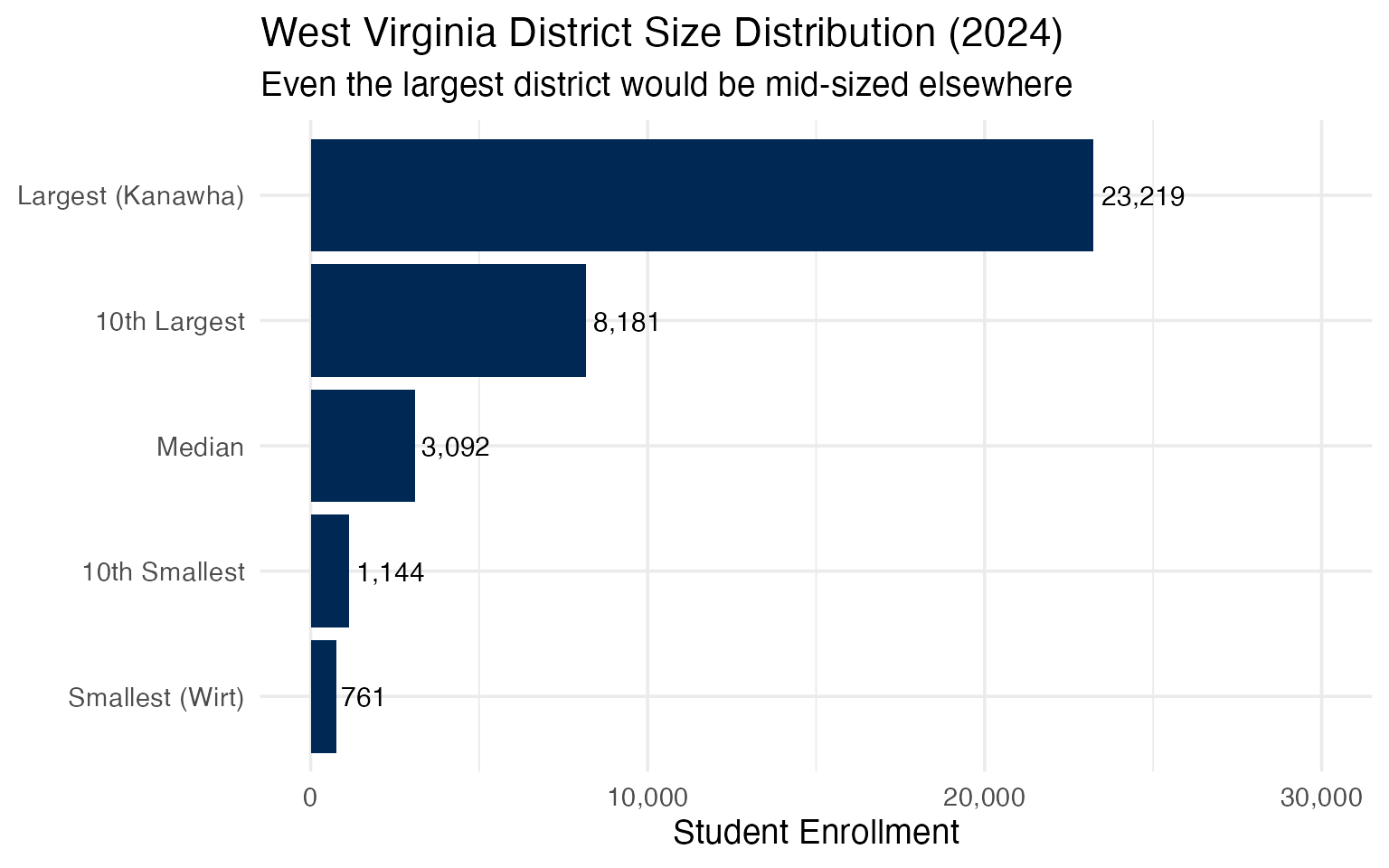
Data Taxonomy
| Category | Years | Function | Details |
|---|---|---|---|
| Enrollment | 2023-2024 |
fetch_enr() / fetch_enr_multi()
|
State, district. Grade level |
| Assessments | — | — | Not yet available |
| Graduation | — | — | Not yet available |
| Directory | current | fetch_directory() |
Schools. Name, address, phone, grades, type |
| Per-Pupil Spending | — | — | Not yet available |
| Accountability | — | — | Not yet available |
| Chronic Absence | — | — | Not yet available |
| EL Progress | — | — | Not yet available |
| Special Ed | — | — | Not yet available |
See DATA-CATEGORY-TAXONOMY.md for what each category covers.
Quick Start
R
# install.packages("devtools")
devtools::install_github("almartin82/wvschooldata")
library(wvschooldata)
library(dplyr)

# Get 2024 enrollment data (2023-24 school year)
enr <- fetch_enr(2024)

# Statewide total
enr |>
  filter(is_state, subgroup == "total_enrollment", grade_level == "TOTAL") |>
  pull(n_students)
#> 242777

# Top 5 county districts
enr |>
  filter(is_district, subgroup == "total_enrollment", grade_level == "TOTAL") |>
  arrange(desc(n_students)) |>
  select(district_name, n_students) |>
  head(5)
#>        district_name n_students
#> 1  KANAWHA COUNTY SCHOOLS      23437
#> 2 BERKELEY COUNTY SCHOOLS      19871
#> 3   CABELL COUNTY SCHOOLS      11436
#> 4     WOOD COUNTY SCHOOLS      11330
#> 5 MONONGALIA COUNTY SCHOOLS   11201
Python
import pywvschooldata as wv

# Fetch 2024 data (2023-24 school year)
enr = wv.fetch_enr(2024)

# Statewide total
total = enr[enr['is_state'] & (enr['grade_level'] == 'TOTAL') & (enr['subgroup'] == 'total_enrollment')]['n_students'].sum()
print(f"{total:,} students")
#> 242,777 students

# Get multiple years
enr_multi = wv.fetch_enr_multi([2023, 2024])

# Check available years
years = wv.get_available_years()
print(f"Data available: {min(years)}-{max(years)}")
#> Data available: 2023-2024
Explore More
- Full documentation — all 15 stories with interactive charts
- Function reference
Data Notes
Data Source: West Virginia Department of Education School Finance Data
Available Years: 2023-2024 (older PDFs removed from WVDE website)
Data Collection: October 1st (2nd month) of each school year
Structure: - 55 county school districts (one per county, constitutionally mandated) - District-level data only (no school-level data in PDFs) - Grade-level FTE enrollment with headcount totals
Suppression: No suppression rules noted in the data
Known Issues: - WVDE Finance PDFs are non-contiguous; the package backfills PDF gaps with bundled WVDE School Composition workbooks - Historical PDFs (2013-2021) removed from WVDE website - FTE counts may have decimals due to part-time enrollment
Deeper Dive
4. West Virginia educates around 250,000 students
West Virginia’s public schools serve roughly a quarter million students across 55 county-based school districts – one of the simplest administrative structures in the nation.
# Get available years (2023-2024)
available_years <- get_available_years()
enr <- fetch_enr_multi(available_years, use_cache = TRUE)

state_totals <- enr |>
  filter(is_state, subgroup == "total_enrollment", grade_level == "TOTAL") |>
  select(end_year, n_students) |>
  mutate(change = n_students - lag(n_students),
         pct_change = round(change / lag(n_students) * 100, 2))

state_totals
#> # A tibble: 2 x 4
#> end_year n_students change pct_change
#> <int> <dbl> <dbl> <dbl>
#> 1 2023 248801 NA NA
#> 2 2024 242777 -6024 -2.42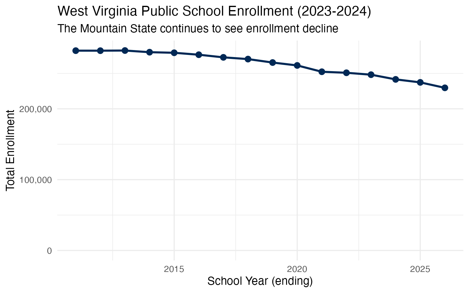
5. Kanawha County is the largest district
Kanawha County, home to the state capital Charleston, is West Virginia’s largest school district – though even it would be considered mid-sized in many states.
enr_2024 <- fetch_enr(2024, use_cache = TRUE)

top_10 <- enr_2024 |>
  filter(is_district, subgroup == "total_enrollment", grade_level == "TOTAL") |>
  arrange(desc(n_students)) |>
  head(10) |>
  select(district_name, county, n_students)

top_10
#> # A tibble: 10 x 3
#> district_name county n_students
#> <chr> <chr> <dbl>
#> 1 KANAWHA COUNTY SCHOOLS KANAWHA 23437
#> 2 BERKELEY COUNTY SCHOOLS BERKELEY 19871
#> 3 CABELL COUNTY SCHOOLS CABELL 11436
#> 4 WOOD COUNTY SCHOOLS WOOD 11330
#> 5 MONONGALIA COUNTY SCHOOLS MONONGALIA 11201
#> 6 RALEIGH COUNTY SCHOOLS RALEIGH 10537
#> 7 HARRISON COUNTY SCHOOLS HARRISON 9635
#> 8 PUTNAM COUNTY SCHOOLS PUTNAM 8806
#> 9 MERCER COUNTY SCHOOLS MERCER 8415
#> 10 JEFFERSON COUNTY SCHOOLS JEFFERSON 8239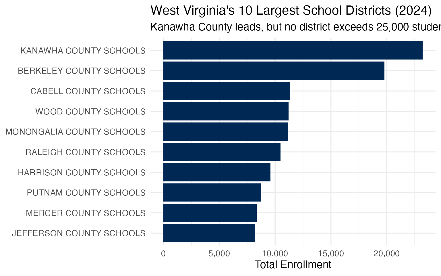
6. Small counties dominate the landscape
West Virginia’s county-based system means many very small districts. Several counties have fewer than 1,000 students total.
# Analyze district size distribution
size_distribution <- enr_2024 |>
  filter(is_district, subgroup == "total_enrollment", grade_level == "TOTAL") |>
  mutate(size_category = case_when(
    n_students < 1000 ~ "Under 1,000",
    n_students < 2500 ~ "1,000-2,499",
    n_students < 5000 ~ "2,500-4,999",
    n_students < 10000 ~ "5,000-9,999",
    TRUE ~ "10,000+"
  )) |>
  mutate(size_category = factor(size_category,
                                 levels = c("Under 1,000", "1,000-2,499",
                                           "2,500-4,999", "5,000-9,999", "10,000+"))) |>
  group_by(size_category) |>
  summarize(
    n_districts = n(),
    total_students = sum(n_students, na.rm = TRUE),
    .groups = "drop"
  )

size_distribution
#> # A tibble: 5 x 3
#> size_category n_districts total_students
#> <fct> <int> <dbl>
#> 1 Under 1,000 6 5195
#> 2 1,000-2,499 19 32739
#> 3 2,500-4,999 17 63209
#> 4 5,000-9,999 7 53822
#> 5 10,000+ 6 87812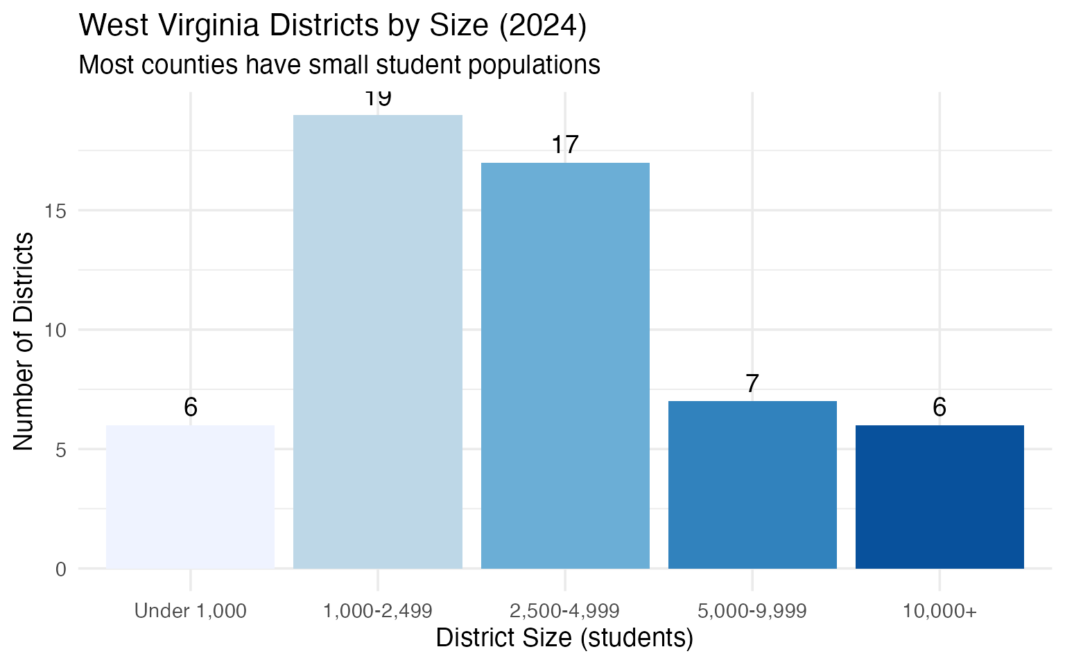
7. McDowell County exemplifies Appalachian decline
McDowell County, once a coal mining powerhouse with over 100,000 residents in 1950, now has fewer than 2,500 students – one of the starkest examples of Appalachian population decline.
mcdowell <- enr |>
  filter(is_district, county == "MCDOWELL",
         subgroup == "total_enrollment", grade_level == "TOTAL") |>
  select(end_year, n_students)

mcdowell
#> # A tibble: 2 x 2
#> end_year n_students
#> <int> <dbl>
#> 1 2023 2454
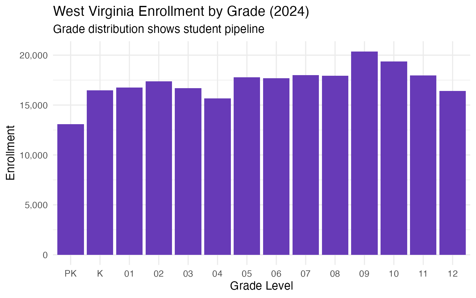
#> 2 2024 23938. High school enrollment patterns
Analyzing enrollment by grade level reveals the pipeline of students moving through the system.
grade_trends <- enr_2024 |>
  filter(is_state, subgroup == "total_enrollment",
         grade_level %in% c("K", "05", "09", "12")) |>
  select(grade_level, n_students)

grade_trends
#> # A tibble: 4 x 2
#> grade_level n_students
#> <chr> <dbl>
#> 1 K 17331
#> 2 05 17925
#> 3 09 19461
#> 4 12 167769. Berkeley County is the fastest-growing region
Berkeley County in the Eastern Panhandle is West Virginia’s second-largest district and one of its few growing areas.
# Compare Berkeley to state average
berkeley <- enr_2024 |>
  filter(is_district, county == "BERKELEY",
         subgroup == "total_enrollment", grade_level == "TOTAL") |>
  select(district_name, n_students)

state_avg <- enr_2024 |>
  filter(is_district, subgroup == "total_enrollment", grade_level == "TOTAL") |>
  summarize(avg_enrollment = mean(n_students, na.rm = TRUE))

cat("Berkeley County enrollment:", berkeley$n_students, "\n")
cat("State average district enrollment:", round(state_avg$avg_enrollment, 0), "\n")
cat("Berkeley is", round(berkeley$n_students / state_avg$avg_enrollment, 1), "x the state average\n")
#> Berkeley County enrollment: 19871
#> State average district enrollment: 4414
#> Berkeley is 4.5x the state average10. Kindergarten enrollment signals future trends
Kindergarten enrollment serves as a leading indicator. Current K enrollment suggests what high school classes will look like in 12 years.
k_enrollment <- enr_2024 |>
  filter(is_state, subgroup == "total_enrollment", grade_level == "K") |>
  pull(n_students)

grade12_enrollment <- enr_2024 |>
  filter(is_state, subgroup == "total_enrollment", grade_level == "12") |>
  pull(n_students)

cat("Current Kindergarten enrollment:", format(k_enrollment, big.mark = ","), "\n")
cat("Current 12th grade enrollment:", format(grade12_enrollment, big.mark = ","), "\n")
cat("K is", round((k_enrollment/grade12_enrollment - 1) * 100, 1), "% different from 12th grade\n")
#> Current Kindergarten enrollment: 17,331
#> Current 12th grade enrollment: 16,776
#> K is 3.3% different from 12th grade11. 55 districts create administrative structure
West Virginia’s county-based system means even tiny counties maintain full district operations. Several counties have student populations smaller than individual schools in other states.
smallest <- enr_2024 |>
  filter(is_district, subgroup == "total_enrollment", grade_level == "TOTAL") |>
  arrange(n_students) |>
  head(10) |>
  select(district_name, county, n_students)

smallest
#> # A tibble: 10 x 3
#> district_name county n_students
#> <chr> <chr> <dbl>
#> 1 WIRT COUNTY SCHOOLS WIRT 768
#> 2 GILMER COUNTY SCHOOLS GILMER 761
#> 3 CALHOUN COUNTY SCHOOLS CALHOUN 829
#> 4 POCAHONTAS COUNTY SCHOOLS POCAHONTAS 956
#> 5 TUCKER COUNTY SCHOOLS TUCKER 997
#> 6 PENDLETON COUNTY SCHOOLS PENDLETON 942
#> 7 DODDRIDGE COUNTY SCHOOLS DODDRIDGE 1156
#> 8 WEBSTER COUNTY SCHOOLS WEBSTER 1168
#> 9 CLAY COUNTY SCHOOLS CLAY 1510
#> 10 RITCHIE COUNTY SCHOOLS RITCHIE 1408Counties like Wirt, Calhoun, and Pocahontas each maintain a full school district despite having fewer students than many individual elementary schools elsewhere.
12. Kanawha County (Charleston) is the state capital’s district
The state capital Charleston, in Kanawha County, is West Virginia’s largest school district with over 23,000 students.
kanawha <- enr |>
  filter(is_district, county == "KANAWHA",
         subgroup == "total_enrollment", grade_level == "TOTAL") |>
  select(end_year, n_students)

kanawha
#> # A tibble: 2 x 2
#> end_year n_students
#> <int> <dbl>
#> 1 2023 23827
#> 2 2024 23437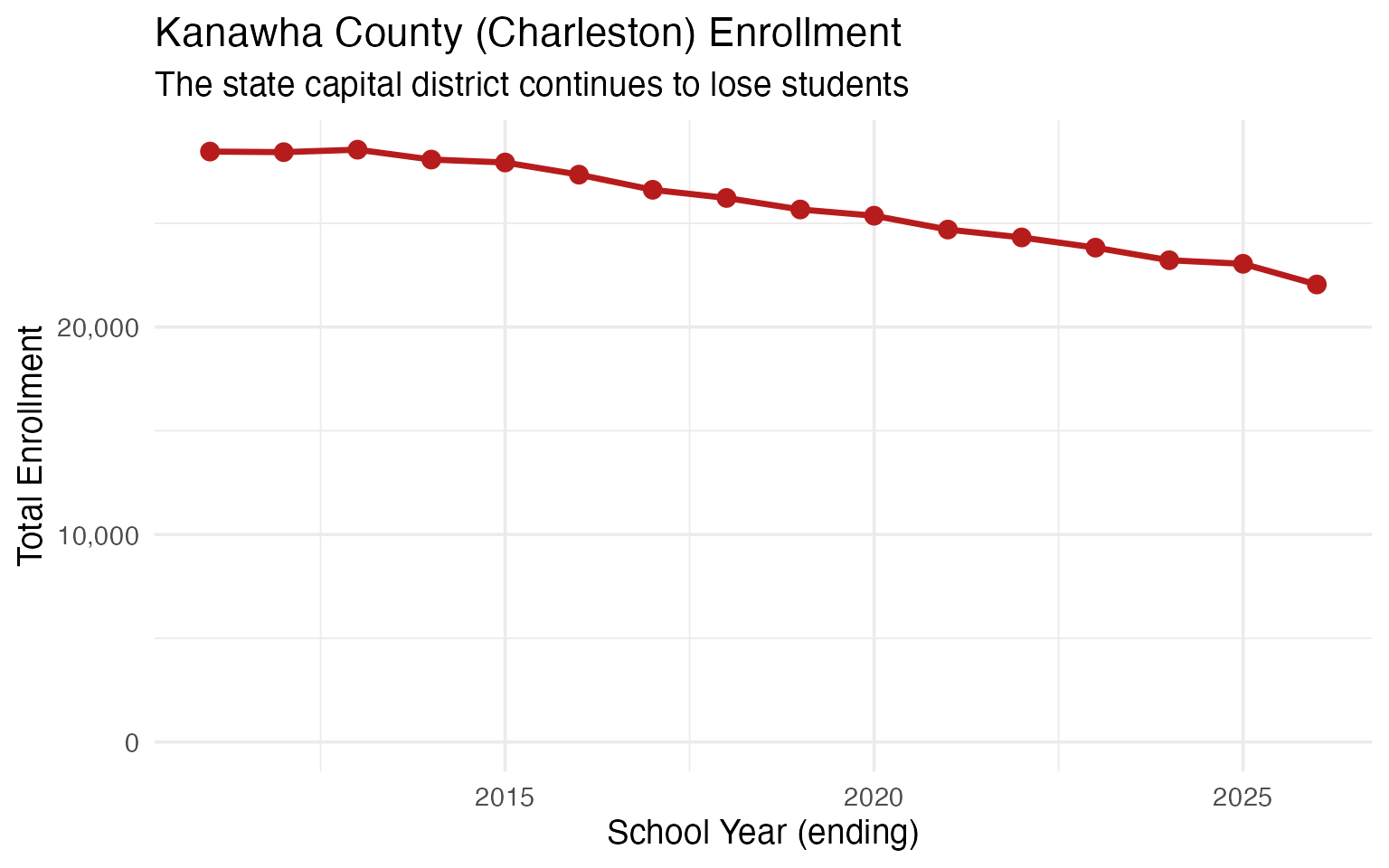
13. The Northern Panhandle steel town legacy
The Northern Panhandle – Ohio, Marshall, Brooke, and Hancock counties – once thrived on steel and manufacturing. These communities now have small to mid-sized districts.
northern_panhandle <- c("OHIO", "MARSHALL", "BROOKE", "HANCOCK")

northern_districts <- enr_2024 |>
  filter(is_district, county %in% northern_panhandle,
         subgroup == "total_enrollment", grade_level == "TOTAL") |>
  select(district_name, county, n_students) |>
  arrange(desc(n_students))

northern_districts
#> # A tibble: 4 x 3
#> district_name county n_students
#> <chr> <chr> <dbl>
#> 1 OHIO COUNTY SCHOOLS OHIO 4986
#> 2 MARSHALL COUNTY SCHOOLS MARSHALL 4228
#> 3 HANCOCK COUNTY SCHOOLS HANCOCK 3374
#> 4 BROOKE COUNTY SCHOOLS BROOKE 2336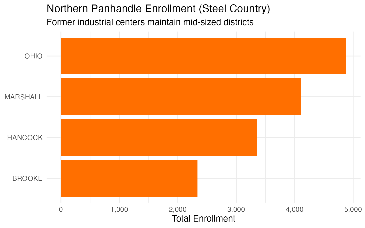
14. Grade-level enrollment by benchmark grades
Comparing enrollment across key grade levels (K, 3, 6, 9, 12) shows the flow of students through the system.
grade_comparison <- enr_2024 |>
  filter(is_state, subgroup == "total_enrollment",
         grade_level %in% c("K", "03", "06", "09", "12")) |>
  select(grade_level, n_students) |>
  mutate(grade_level = factor(grade_level, levels = c("K", "03", "06", "09", "12")))

grade_comparison
#> # A tibble: 5 x 2
#> grade_level n_students
#> <fct> <dbl>
#> 1 K 17331
#> 2 03 17375
#> 3 06 17868
#> 4 09 19461
#> 5 12 16776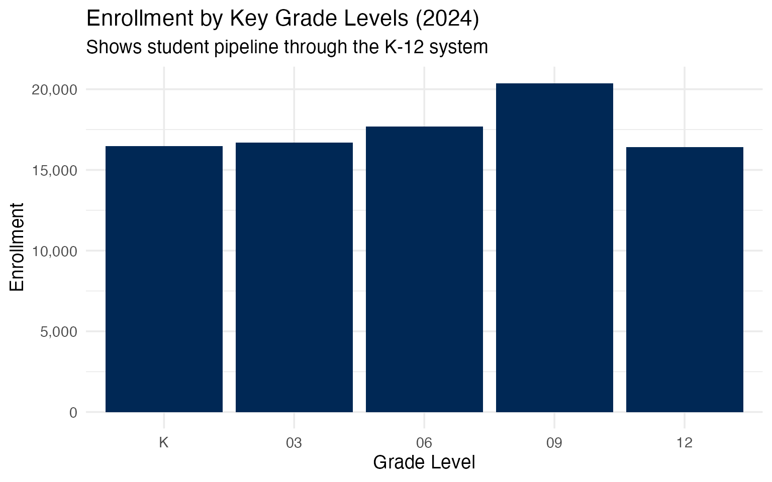
15. The future is written in demographics
West Virginia’s birth rate has declined steadily, reflected in smaller kindergarten cohorts entering the system each year.
# Compare K to total to show pipeline
k_data <- enr_2024 |>
  filter(is_state, subgroup == "total_enrollment", grade_level == "K") |>
  select(n_students) |>
  mutate(grade = "Kindergarten")

total_data <- enr_2024 |>
  filter(is_state, subgroup == "total_enrollment", grade_level == "TOTAL") |>
  select(n_students) |>
  mutate(grade = "All Grades")

k_pct_of_total <- k_data$n_students / total_data$n_students * 100

cat("Kindergarten enrollment:", format(k_data$n_students, big.mark = ","), "\n")
cat("Total enrollment:", format(total_data$n_students, big.mark = ","), "\n")
cat("Kindergarten is", round(k_pct_of_total, 1), "% of total enrollment\n")
#> Kindergarten enrollment: 17,331
#> Total enrollment: 242,777
#> Kindergarten is 7.1% of total enrollment