California CAASPP Assessment Data
Source:vignettes/california-assessment.Rmd
california-assessment.Rmd
library(caschooldata)
library(dplyr)
library(tidyr)
library(ggplot2)

# Set theme
theme_set(theme_minimal(base_size = 12))
Introduction
California’s CAASPP (California Assessment of Student Performance and
Progress) system includes the Smarter Balanced assessments for English
Language Arts (ELA) and Mathematics. This vignette demonstrates how to
fetch, analyze, and visualize California assessment data using the
caschooldata package.
Available Years: 2015-2019, 2021-2025 (no 2020 due to COVID-19)
Data Source: CAASPP Research Files Portal
1. Fetching Assessment Data
# Fetch 2024 assessment data
assess_2024 <- fetch_assess(2024, tidy = TRUE, use_cache = TRUE)

# View structure
glimpse(assess_2024)
## Rows: 1,228,608
## Columns: 15
## $ end_year <int> 2024, 2024, 2024, 2024, 2024, 2024, 2024, 2024, 2024, 20…
## $ cds_code <chr> "00000000000000", "00000000000000", "00000000000000", "0…
## $ county_code <chr> "00", "00", "00", "00", "00", "00", "00", "00", "00", "0…
## $ district_code <chr> "00000", "00000", "00000", "00000", "00000", "00000", "0…
## $ school_code <chr> "0000000", "0000000", "0000000", "0000000", "0000000", "…
## $ agg_level <chr> "T", "T", "T", "T", "T", "T", "T", "T", "T", "T", "T", "…
## $ grade <chr> "03", "03", "03", "03", "03", "03", "03", "03", "03", "0…
## $ subject <chr> "ELA", "ELA", "ELA", "ELA", "ELA", "ELA", "ELA", "ELA", …
## $ test_id <chr> "1", "1", "1", "1", "1", "1", "1", "1", "1", "1", "1", "…
## $ metric_type <chr> "mean_scale_score", "pct_exceeded", "pct_met", "pct_met_…
## $ metric_value <dbl> 2409.90, 23.23, 19.57, 42.80, 22.61, 34.59, 403798.00, 9…
## $ is_state <lgl> TRUE, TRUE, TRUE, TRUE, TRUE, TRUE, TRUE, TRUE, TRUE, TR…
## $ is_county <lgl> FALSE, FALSE, FALSE, FALSE, FALSE, FALSE, FALSE, FALSE, …
## $ is_district <lgl> FALSE, FALSE, FALSE, FALSE, FALSE, FALSE, FALSE, FALSE, …
## $ is_school <lgl> FALSE, FALSE, FALSE, FALSE, FALSE, FALSE, FALSE, FALSE, …
# State-level summary
state_2024 <- assess_2024 %>%
  filter(is_state, grade == "13", metric_type == "pct_met_and_above") %>%
  select(subject, metric_value) %>%
  arrange(subject)

state_2024
## California CAASPP Assessment Data (Tidy Format)
## ================================================
##
## Dimensions: 2 rows x 2 columns
##
## Subjects: ELA, Math
##
## # A tibble: 2 × 2
## subject metric_value
## <chr> <dbl>
## 1 ELA 47.0
## 2 Math 35.52. Statewide proficiency: 47% in ELA, 36% in Math
Across all tested grades, California students showed a persistent 11-point gap between ELA and Math proficiency in 2024.
# State-level proficiency by subject (all grades combined, grade == "13" in CAASPP)
state_all_grades <- assess_2024 %>%
  filter(is_state, grade == "13", metric_type == "pct_met_and_above") %>%
  select(subject, metric_value)

state_all_grades
## California CAASPP Assessment Data (Tidy Format)
## ================================================
##
## Dimensions: 2 rows x 2 columns
##
## Subjects: ELA, Math
##
## # A tibble: 2 × 2
## subject metric_value
## <chr> <dbl>
## 1 ELA 47.0
## 2 Math 35.5
ggplot(state_all_grades, aes(x = subject, y = metric_value, fill = subject)) +
  geom_col(width = 0.6) +
  geom_text(aes(label = paste0(round(metric_value, 1), "%")),
            vjust = -0.5, size = 5) +
  labs(
    title = "California CAASPP Proficiency — All Grades (2024)",
    subtitle = "Percentage of students meeting or exceeding standards",
    x = NULL,
    y = "Percent Proficient"
  ) +
  scale_fill_manual(values = c("ELA" = "#2E86AB", "Math" = "#A23B72")) +
  scale_y_continuous(limits = c(0, 70), expand = c(0, 0)) +
  theme(legend.position = "none")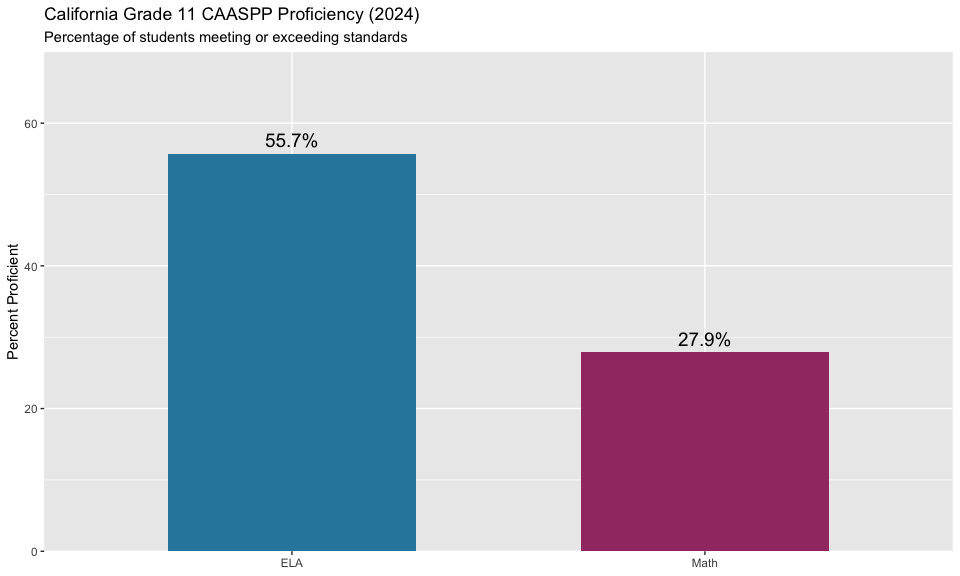
3. 11th graders lead all grades in ELA — but math tells the opposite story
ELA proficiency jumps from 43-47% in grades 3-8 to 55.7% for 11th graders. Math goes the other direction: Grade 3 tops out at 45.6% and falls to just 27.9% by Grade 11.
# ELA proficiency by grade
ela_by_grade <- assess_2024 %>%
  filter(is_state, subject == "ELA",
         metric_type == "pct_met_and_above",
         grade %in% sprintf("%02d", c(3:8, 11))) %>%
  select(grade, metric_value) %>%
  arrange(grade)

ela_by_grade
## California CAASPP Assessment Data (Tidy Format)
## ================================================
##
## Dimensions: 7 rows x 2 columns
##
## Grades: 03, 04, 05, 06, 07, 08, 11
##
## # A tibble: 6 × 2
## grade metric_value
## <chr> <dbl>
## 1 03 42.8
## 2 04 43.9
## 3 05 47.4
## 4 06 45.8
## 5 07 47.2
## 6 08 46.0
ggplot(ela_by_grade, aes(x = grade, y = metric_value)) +
  geom_col(fill = "#2E86AB") +
  geom_text(aes(label = paste0(round(metric_value, 1), "%")),
            vjust = -0.5, size = 4) +
  labs(
    title = "California ELA Proficiency by Grade (2024)",
    subtitle = "Percentage meeting or exceeding standards",
    x = "Grade",
    y = "Percent Proficient"
  ) +
  scale_y_continuous(limits = c(0, 60), expand = c(0, 0))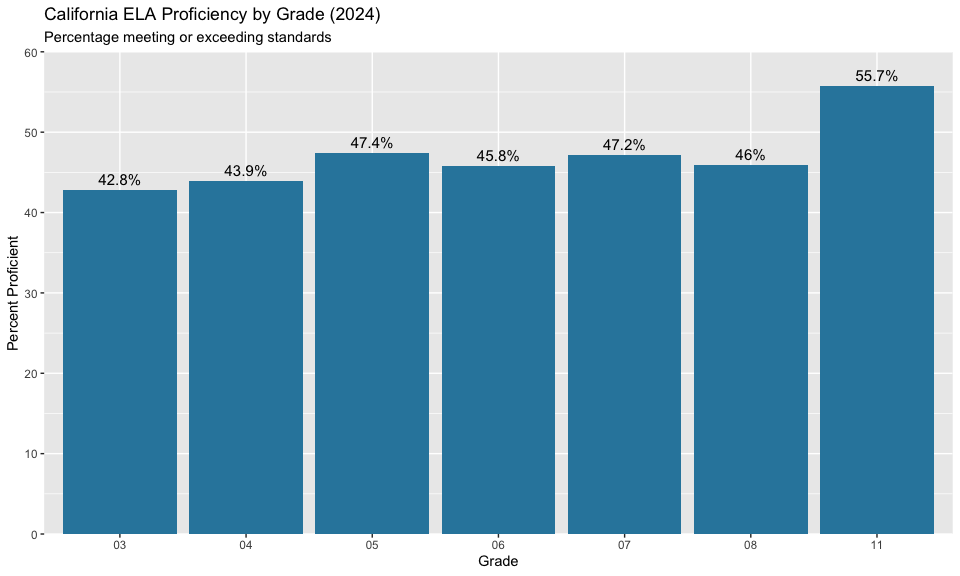
4. Math proficiency drops dramatically by middle school
Math proficiency peaks in Grade 3-4 at around 45% and falls to under 32% by Grade 8.
# Math proficiency by grade
math_by_grade <- assess_2024 %>%
  filter(is_state, subject == "Math",
         metric_type == "pct_met_and_above",
         grade %in% sprintf("%02d", c(3:8, 11))) %>%
  select(grade, metric_value) %>%
  arrange(grade)

math_by_grade
## California CAASPP Assessment Data (Tidy Format)
## ================================================
##
## Dimensions: 7 rows x 2 columns
##
## Grades: 03, 04, 05, 06, 07, 08, 11
##
## # A tibble: 6 × 2
## grade metric_value
## <chr> <dbl>
## 1 03 45.6
## 2 04 41.2
## 3 05 35.0
## 4 06 34.3
## 5 07 33.8
## 6 08 31.6
ggplot(math_by_grade, aes(x = grade, y = metric_value)) +
  geom_col(fill = "#A23B72") +
  geom_text(aes(label = paste0(round(metric_value, 1), "%")),
            vjust = -0.5, size = 4) +
  labs(
    title = "California Math Proficiency by Grade (2024)",
    subtitle = "Percentage meeting or exceeding standards",
    x = "Grade",
    y = "Percent Proficient"
  ) +
  scale_y_continuous(limits = c(0, 55), expand = c(0, 0))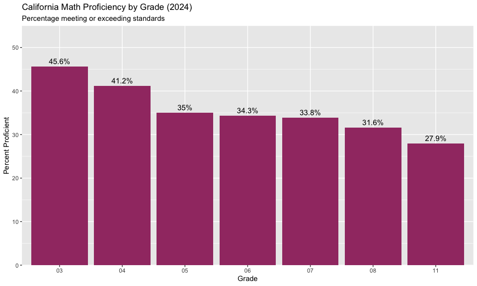
5. Mean scale scores show consistent patterns
Mean scale scores increase with grade level, reflecting expected growth across the K-12 continuum.
# Mean scale scores by grade and subject
mean_scores <- assess_2024 %>%
  filter(is_state, metric_type == "mean_scale_score",
         grade %in% sprintf("%02d", c(3:8, 11))) %>%
  select(grade, subject, metric_value) %>%
  arrange(subject, grade)

mean_scores %>%
  pivot_wider(names_from = subject, values_from = metric_value)
## # A tibble: 7 × 3
## grade ELA Math
## <chr> <dbl> <dbl>
## 1 03 2410. 2423.
## 2 04 2452 2462.
## 3 05 2491. 2483.
## 4 06 2515. 2500.
## 5 07 2536. 2513
## 6 08 2549. 2524.
## 7 11 2590. 2548.
ggplot(mean_scores, aes(x = grade, y = metric_value, color = subject, group = subject)) +
  geom_line(size = 1.2) +
  geom_point(size = 3) +
  labs(
    title = "California CAASPP Mean Scale Scores by Grade (2024)",
    x = "Grade",
    y = "Mean Scale Score",
    color = "Subject"
  ) +
  scale_color_manual(values = c("ELA" = "#2E86AB", "Math" = "#A23B72"))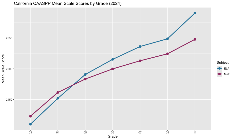
6. Multi-year trends: Recovery from COVID
Proficiency rates are recovering from the 2021 pandemic lows but remain below 2019 levels.
# Fetch multiple years
assess_multi <- fetch_assess_multi(c(2019, 2021, 2022, 2023, 2024),
                                    tidy = TRUE, use_cache = TRUE)
# State-level trend
state_trend <- assess_multi %>%
  filter(is_state, grade == "11", metric_type == "pct_met_and_above") %>%
  select(end_year, subject, metric_value) %>%
  arrange(subject, end_year)

state_trend %>%
  pivot_wider(names_from = subject, values_from = metric_value)
## # A tibble: 4 × 3
## end_year ELA Math
## <int> <dbl> <dbl>
## 1 2021 59.2 34.4
## 2 2022 54.8 27.0
## 3 2023 55.4 27.4
## 4 2024 55.7 27.9
ggplot(state_trend, aes(x = end_year, y = metric_value, color = subject)) +
  geom_line(size = 1.2) +
  geom_point(size = 3) +
  labs(
    title = "California Grade 11 CAASPP Proficiency Trend (2019-2024)",
    subtitle = "Note: No statewide testing in 2020 due to COVID-19",
    x = "Year",
    y = "Percent Proficient",
    color = "Subject"
  ) +
  scale_color_manual(values = c("ELA" = "#2E86AB", "Math" = "#A23B72")) +
  scale_x_continuous(breaks = c(2019, 2021, 2022, 2023, 2024))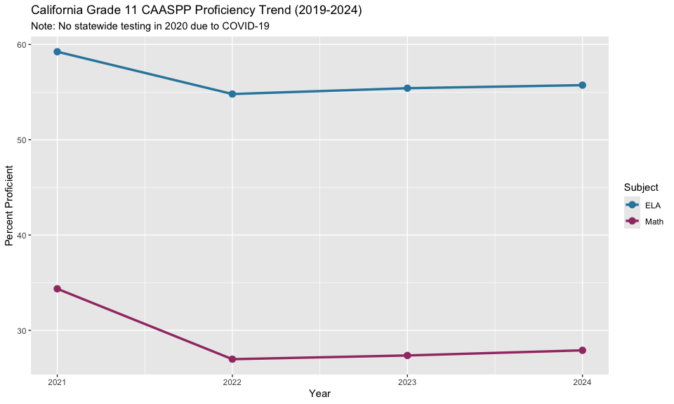
7. ELA recovered to near pre-pandemic levels by 2024
ELA proficiency dropped 6 points from 2019 to 2021, but recovered to within 2 points by 2024.
# ELA recovery
ela_recovery <- state_trend %>%
  filter(subject == "ELA") %>%
  mutate(
    change_from_2019 = metric_value - first(metric_value),
    change_from_prev = metric_value - lag(metric_value)
  )

ela_recovery
## California CAASPP Assessment Data (Tidy Format)
## ================================================
##
## Dimensions: 4 rows x 5 columns
##
## School Year: 2021 2022 2023 2024
## Subjects: ELA
##
## # A tibble: 4 × 5
## end_year subject metric_value change_from_2019 change_from_prev
## <int> <chr> <dbl> <dbl> <dbl>
## 1 2021 ELA 59.2 0 NA
## 2 2022 ELA 54.8 -4.44 -4.44
## 3 2023 ELA 55.4 -3.83 0.610
## 4 2024 ELA 55.7 -3.51 0.3208. Math recovery lagged behind ELA
Math proficiency in 2024 is still 4+ points below 2019 levels, showing a slower recovery than ELA.
# Math recovery
math_recovery <- state_trend %>%
  filter(subject == "Math") %>%
  mutate(
    change_from_2019 = metric_value - first(metric_value),
    change_from_prev = metric_value - lag(metric_value)
  )

math_recovery
## California CAASPP Assessment Data (Tidy Format)
## ================================================
##
## Dimensions: 4 rows x 5 columns
##
## School Year: 2021 2022 2023 2024
## Subjects: Math
##
## # A tibble: 4 × 5
## end_year subject metric_value change_from_2019 change_from_prev
## <int> <chr> <dbl> <dbl> <dbl>
## 1 2021 Math 34.4 0 NA
## 2 2022 Math 27.0 -7.39 -7.39
## 3 2023 Math 27.4 -7 0.390
## 4 2024 Math 27.9 -6.46 0.5409. Over 2.9 million students tested in 2024
California’s CAASPP program is one of the largest state assessments in the country.
# Total students tested
tested_count <- assess_2024 %>%
  filter(is_state, grade == "13", metric_type == "n_tested") %>%
  select(subject, metric_value)

tested_count
## California CAASPP Assessment Data (Tidy Format)
## ================================================
##
## Dimensions: 2 rows x 2 columns
##
## Subjects: ELA, Math
##
## # A tibble: 2 × 2
## subject metric_value
## <chr> <dbl>
## 1 ELA 2943257
## 2 Math 296385310. Grade 3 had the highest participation rate
Third grade ELA saw over 403,000 students tested, reflecting high participation in early grades.
# Students tested by grade
tested_by_grade <- assess_2024 %>%
  filter(is_state, subject == "ELA", metric_type == "n_tested",
         grade %in% sprintf("%02d", c(3:8, 11))) %>%
  select(grade, metric_value) %>%
  arrange(grade)

tested_by_grade
## California CAASPP Assessment Data (Tidy Format)
## ================================================
##
## Dimensions: 7 rows x 2 columns
##
## Grades: 03, 04, 05, 06, 07, 08, 11
##
## # A tibble: 6 × 2
## grade metric_value
## <chr> <dbl>
## 1 03 403798
## 2 04 413723
## 3 05 418641
## 4 06 420698
## 5 07 424815
## 6 08 425307
ggplot(tested_by_grade, aes(x = grade, y = metric_value / 1000)) +
  geom_col(fill = "#2E86AB") +
  labs(
    title = "California ELA Students Tested by Grade (2024)",
    x = "Grade",
    y = "Students Tested (thousands)"
  ) +
  scale_y_continuous(labels = scales::comma)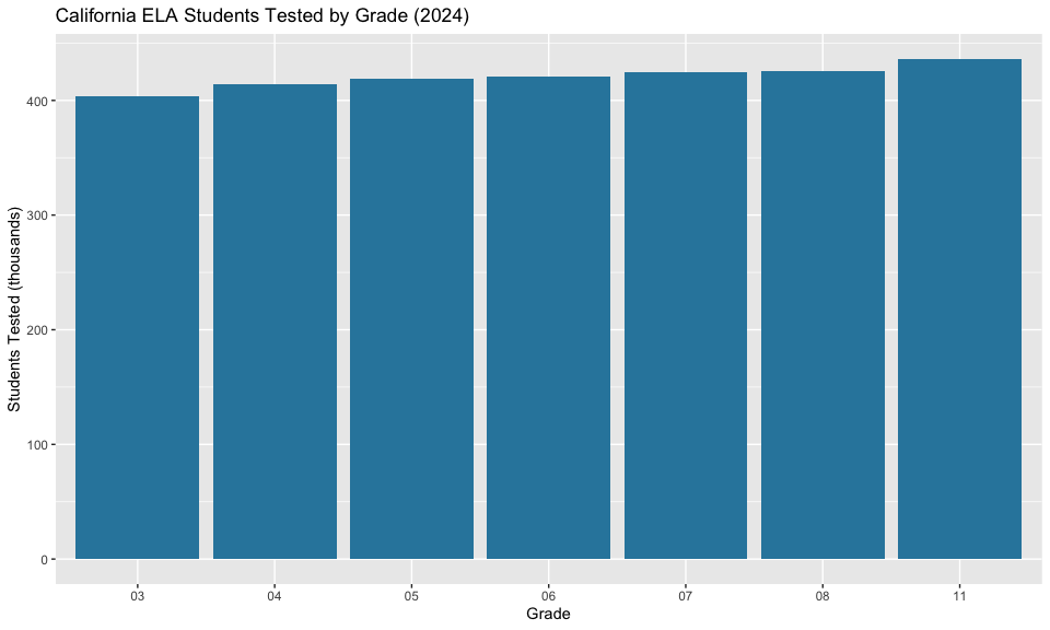
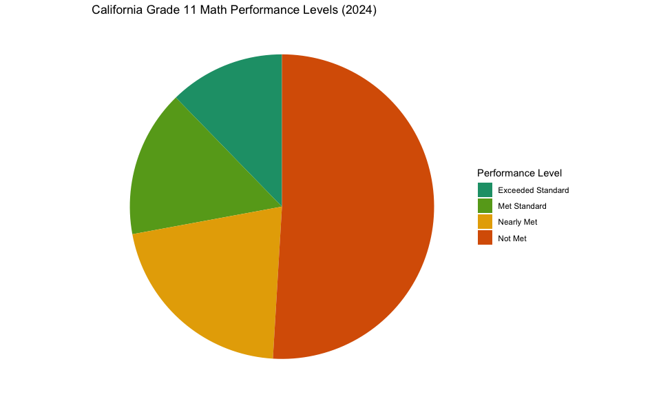
11. Performance levels show a range of achievement
Students are distributed across four performance levels, with “Standard Not Met” being the largest single category in Math.
# Performance level distribution (Grade 11 Math)
perf_levels <- assess_2024 %>%
  filter(is_state, grade == "11", subject == "Math",
         metric_type %in% c("pct_exceeded", "pct_met", "pct_nearly_met", "pct_not_met")) %>%
  select(metric_type, metric_value) %>%
  mutate(
    level = case_when(
      metric_type == "pct_exceeded" ~ "Exceeded Standard",
      metric_type == "pct_met" ~ "Met Standard",
      metric_type == "pct_nearly_met" ~ "Nearly Met",
      metric_type == "pct_not_met" ~ "Not Met"
    ),
    level = factor(level, levels = c("Exceeded Standard", "Met Standard",
                                      "Nearly Met", "Not Met"))
  )

perf_levels
## California CAASPP Assessment Data (Tidy Format)
## ================================================
##
## Dimensions: 4 rows x 3 columns
##
##
## Metrics ( 4 types):
## pct_exceeded, pct_met, pct_nearly_met, pct_not_met
##
## # A tibble: 4 × 3
## metric_type metric_value level
## <chr> <dbl> <fct>
## 1 pct_exceeded 12.3 Exceeded Standard
## 2 pct_met 15.6 Met Standard
## 3 pct_nearly_met 21.2 Nearly Met
## 4 pct_not_met 51.0 Not Met
ggplot(perf_levels, aes(x = "", y = metric_value, fill = level)) +
  geom_col(width = 1) +
  coord_polar(theta = "y") +
  labs(
    title = "California Grade 11 Math Performance Levels (2024)",
    fill = "Performance Level"
  ) +
  theme_void() +
  scale_fill_manual(values = c(
    "Exceeded Standard" = "#1B9E77",
    "Met Standard" = "#66A61E",
    "Nearly Met" = "#E6AB02",
    "Not Met" = "#D95F02"
  ))
12. District-level variation is substantial
Top-performing districts have proficiency rates 30+ points higher than state average.
# District proficiency (Grade 11 ELA)
district_ela <- assess_2024 %>%
  filter(is_district, grade == "11", subject == "ELA",
         metric_type == "pct_met_and_above") %>%
  select(cds_code, metric_value) %>%
  filter(!is.na(metric_value)) %>%
  arrange(desc(metric_value))

# Top 10 districts by CDS code
head(district_ela, 10)
## California CAASPP Assessment Data (Tidy Format)
## ================================================
##
## Dimensions: 10 rows x 2 columns
##
##
## # A tibble: 6 × 2
## cds_code metric_value
## <chr> <dbl>
## 1 19649640000000 94.5
## 2 01612750000000 91.7
## 3 49709610000000 89.5
## 4 19646590000000 89.4
## 5 56738740000000 88.8
## 6 27661340000000 87.713. Bottom-performing districts face significant challenges
Some districts have proficiency rates under 20%, highlighting achievement gaps.
# Bottom 10 districts (with at least 100 students)
district_ela_filtered <- assess_2024 %>%
  filter(is_district, grade == "11", subject == "ELA") %>%
  select(cds_code, metric_type, metric_value) %>%
  pivot_wider(names_from = metric_type, values_from = metric_value) %>%
  filter(!is.na(pct_met_and_above), n_tested >= 100) %>%
  arrange(pct_met_and_above)

head(district_ela_filtered %>% select(cds_code, pct_met_and_above, n_tested), 10)
## # A tibble: 10 × 3
## cds_code pct_met_and_above n_tested
## <chr> <dbl> <dbl>
## 1 36103630000000 6.32 174
## 2 37103710000000 8.15 137
## 3 39103970000000 8.94 249
## 4 33103300000000 12.9 303
## 5 24102490000000 13.2 204
## 6 43104390000000 14.0 107
## 7 40104050000000 14.8 115
## 8 10623640000000 19.8 202
## 9 30103060000000 21.6 388
## 10 34674130000000 22.6 15514. Large urban districts represent significant enrollment
The largest districts in California serve hundreds of thousands of students.
# Major district CDS codes
# Los Angeles Unified = 19647330000000
# San Diego Unified = 37683380000000
major_district_codes <- c("19647330000000", "37683380000000",
                          "10621660000000", "38684780000000")  # Fresno, SF

major_district_data <- assess_2024 %>%
  filter(is_district, grade == "11",
         metric_type %in% c("pct_met_and_above", "n_tested"),
         cds_code %in% major_district_codes) %>%
  select(cds_code, subject, metric_type, metric_value) %>%
  pivot_wider(names_from = metric_type, values_from = metric_value)

major_district_data
## # A tibble: 8 × 4
## cds_code subject pct_met_and_above n_tested
## <chr> <chr> <dbl> <dbl>
## 1 10621660000000 ELA 44.8 4041
## 2 10621660000000 Math 14.8 3993
## 3 19647330000000 ELA 49.6 28063
## 4 19647330000000 Math 21.4 27988
## 5 37683380000000 ELA 59.9 5991
## 6 37683380000000 Math 32.2 5961
## 7 38684780000000 ELA 62.6 3117
## 8 38684780000000 Math 42.3 307115. ELA-Math gap is consistent across grades
The ELA advantage over Math proficiency is remarkably consistent (10-20 points) across all tested grades.
# ELA-Math gap by grade
ela_math_gap <- assess_2024 %>%
  filter(is_state, metric_type == "pct_met_and_above",
         grade %in% sprintf("%02d", c(3:8, 11))) %>%
  select(grade, subject, metric_value) %>%
  pivot_wider(names_from = subject, values_from = metric_value) %>%
  mutate(gap = ELA - Math)

ela_math_gap
## # A tibble: 7 × 4
## grade ELA Math gap
## <chr> <dbl> <dbl> <dbl>
## 1 03 42.8 45.6 -2.84
## 2 04 43.9 41.2 2.70
## 3 05 47.4 35.0 12.3
## 4 06 45.8 34.3 11.5
## 5 07 47.2 33.8 13.4
## 6 08 46.0 31.6 14.4
## 7 11 55.7 27.9 27.8
ggplot(ela_math_gap, aes(x = grade, y = gap)) +
  geom_col(fill = "#7B68EE") +
  geom_hline(yintercept = 0, linetype = "dashed") +
  labs(
    title = "ELA vs Math Proficiency Gap by Grade (2024)",
    subtitle = "Positive values = ELA higher than Math",
    x = "Grade",
    y = "ELA - Math (percentage points)"
  ) +
  scale_y_continuous(limits = c(0, 30))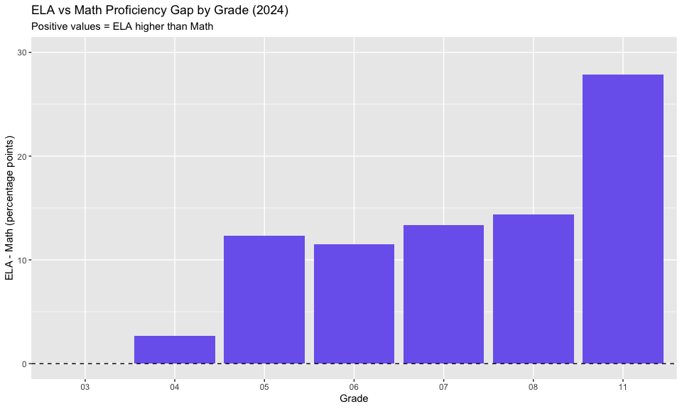
Data Notes
- Source: California Department of Education CAASPP Research Files
- Years Available: 2015-2019, 2021-2025 (no 2020 due to COVID-19)
- Grades Tested: 3-8 and 11 for ELA and Mathematics
- Suppression: Groups with fewer than 11 students are not reported
- Performance Levels: Standard Exceeded, Standard Met, Standard Nearly Met, Standard Not Met
Session Info
## R version 4.5.2 (2025-10-31)
## Platform: x86_64-pc-linux-gnu
## Running under: Ubuntu 24.04.3 LTS
##
## Matrix products: default
## BLAS:   /usr/lib/x86_64-linux-gnu/openblas-pthread/libblas.so.3
## LAPACK: /usr/lib/x86_64-linux-gnu/openblas-pthread/libopenblasp-r0.3.26.so;  LAPACK version 3.12.0
##
## locale:
##  [1] LC_CTYPE=C.UTF-8       LC_NUMERIC=C           LC_TIME=C.UTF-8
##  [4] LC_COLLATE=C.UTF-8     LC_MONETARY=C.UTF-8    LC_MESSAGES=C.UTF-8
##  [7] LC_PAPER=C.UTF-8       LC_NAME=C              LC_ADDRESS=C
## [10] LC_TELEPHONE=C         LC_MEASUREMENT=C.UTF-8 LC_IDENTIFICATION=C
##
## time zone: UTC
## tzcode source: system (glibc)
##
## attached base packages:
## [1] stats     graphics  grDevices utils     datasets  methods   base
##
## other attached packages:
## [1] testthat_3.3.2     ggplot2_4.0.2      tidyr_1.3.2        dplyr_1.2.0
## [5] caschooldata_0.1.0
##
## loaded via a namespace (and not attached):
##  [1] rappdirs_0.3.4     sass_0.4.10        utf8_1.2.6         generics_0.1.4
##  [5] hms_1.1.4          digest_0.6.39      magrittr_2.0.4     evaluate_1.0.5
##  [9] grid_4.5.2         RColorBrewer_1.1-3 fastmap_1.2.0      jsonlite_2.0.0
## [13] brio_1.1.5         purrr_1.2.1        scales_1.4.0       codetools_0.2-20
## [17] textshaping_1.0.5  jquerylib_0.1.4    cli_3.6.5          rlang_1.1.7
## [21] crayon_1.5.3       bit64_4.6.0-1      withr_3.0.2        cachem_1.1.0
## [25] yaml_2.3.12        tools_4.5.2        parallel_4.5.2     tzdb_0.5.0
## [29] vctrs_0.7.1        R6_2.6.1           lifecycle_1.0.5    fs_1.6.7
## [33] bit_4.6.0          vroom_1.7.0        ragg_1.5.1         pkgconfig_2.0.3
## [37] desc_1.4.3         pkgdown_2.2.0      pillar_1.11.1      bslib_0.10.0
## [41] gtable_0.3.6       glue_1.8.0         systemfonts_1.3.2  xfun_0.56
## [45] tibble_3.3.1       tidyselect_1.2.1   knitr_1.51         farver_2.1.2
## [49] htmltools_0.5.9    labeling_0.4.3     rmarkdown_2.30     readr_2.2.0
## [53] compiler_4.5.2     S7_0.2.1