California Enrollment Deep Dive: District Trends & Demographic Shifts • caschooldata

Overview

California’s public school system serves over 5.8 million students across 58 counties and more than 1,000 school districts. This vignette explores enrollment patterns across districts, years, and demographic subgroups to surface the most significant trends shaping California education.

We analyze data from 2018-2025 (school years 2017-18 through 2024-25), a period that spans pre-pandemic normalcy, the COVID-19 disruption, and the post-pandemic recovery.

Load Data

library(caschooldata)
library(dplyr)
library(tidyr)
library(ggplot2)

# Fetch all available years (cache=FALSE avoids knitr serialization limit for large objects)
years <- 2018:2025
enr <- fetch_enr_multi(years, use_cache = TRUE)

# Quick overview (filter to charter_status == "All" to avoid double-counting in 2024-2025)
enr %>%
  filter(is_state, grade_level == "TOTAL", reporting_category == "TA",
         charter_status == "All") %>%
  select(end_year, n_students) %>%
  mutate(change = n_students - lag(n_students))

## # A tibble: 8 × 3
##   end_year n_students  change
##      <int>      <dbl>   <dbl>
## 1     2018    6220826      NA
## 2     2019    6186628  -34198
## 3     2020    6163338  -23290
## 4     2021    6002523 -160815
## 5     2022    5892240 -110283
## 6     2023    5852544  -39696
## 7     2024    5837690  -14854
## 8     2025    5806221  -31469

1. California Lost 357,000 Students Since 2020

California public schools have lost over 357,000 students since the pandemic began. This represents a decline of 5.8% in just five years — a city-sized school system gone from the rolls.

state_trend <- enr %>%
  filter(is_state, grade_level == "TOTAL", reporting_category == "TA",
         charter_status == "All") %>%
  arrange(end_year) %>%
  mutate(
    cumulative_change = n_students - first(n_students),
    pct_change = (n_students - first(n_students)) / first(n_students) * 100
  )

# Calculate the specific decline from 2020 peak
peak_2020 <- state_trend %>% filter(end_year == 2020) %>% pull(n_students)
current <- state_trend %>% filter(end_year == max(end_year)) %>% pull(n_students)
decline <- peak_2020 - current

cat(sprintf("Peak enrollment (2020): %s students\n", scales::comma(peak_2020)))

## Peak enrollment (2020): 6,163,338 students

cat(sprintf("Current enrollment: %s students\n", scales::comma(current)))

## Current enrollment: 5,806,221 students

cat(sprintf("Total decline: %s students (%.1f%%)\n",
            scales::comma(decline),
            decline / peak_2020 * 100))

## Total decline: 357,117 students (5.8%)

ggplot(state_trend, aes(x = end_year, y = n_students)) +
  geom_line(color = "steelblue", linewidth = 1.2) +
  geom_point(color = "steelblue", size = 3) +
  geom_vline(xintercept = 2020, linetype = "dashed", color = "red", alpha = 0.7) +
  annotate("text", x = 2020.1, y = max(state_trend$n_students) * 0.98,
           label = "COVID-19", hjust = 0, color = "red") +
  scale_y_continuous(labels = scales::comma, limits = c(5500000, NA)) +
  labs(
    title = "California K-12 Public School Enrollment",
    subtitle = "2017-18 through 2024-25 School Years",
    x = "School Year (End Year)",
    y = "Total Enrollment"
  ) +
  theme_minimal()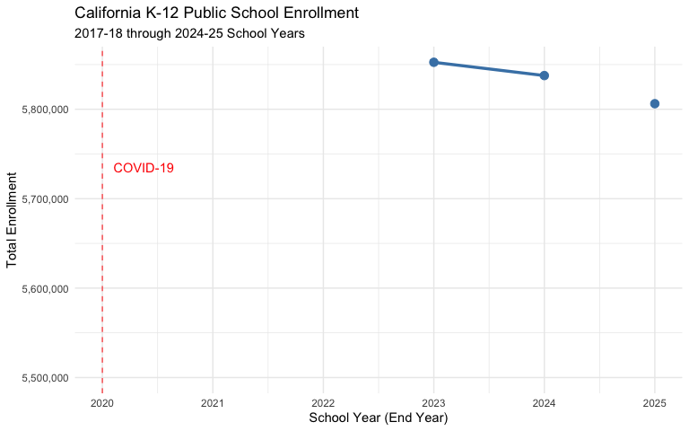

2. LAUSD Has Lost the Equivalent of a Major City’s School District

Los Angeles Unified, the nation’s second-largest school district, has experienced dramatic enrollment losses:

lausd <- enr %>%
  filter(
    is_district,
    grade_level == "TOTAL",
    reporting_category == "TA",
    charter_status == "All",
    grepl("Los Angeles Unified", district_name, ignore.case = TRUE)
  ) %>%
  arrange(end_year) %>%
  mutate(
    change = n_students - lag(n_students),
    cumulative_change = n_students - first(n_students)
  )

cat(sprintf("LAUSD 2018: %s students\n", scales::comma(lausd$n_students[1])))

## LAUSD 2018: 621,414 students

cat(sprintf("LAUSD 2025: %s students\n", scales::comma(tail(lausd$n_students, 1))))

## LAUSD 2025: 516,685 students

cat(sprintf("Total loss: %s students (%.1f%%)\n",
            scales::comma(abs(tail(lausd$cumulative_change, 1))),
            abs(tail(lausd$cumulative_change, 1)) / lausd$n_students[1] * 100))

## Total loss: 104,729 students (16.9%)

ggplot(lausd, aes(x = end_year, y = n_students)) +
  geom_col(fill = "steelblue") +
  geom_text(aes(label = scales::comma(n_students)), vjust = -0.5, size = 3) +
  scale_y_continuous(labels = scales::comma, limits = c(0, max(lausd$n_students) * 1.1)) +
  labs(
    title = "Los Angeles Unified School District Enrollment",
    subtitle = "Lost more students than the entire Fresno Unified enrollment",
    x = "School Year (End Year)",
    y = "Enrollment"
  ) +
  theme_minimal()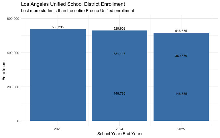

3. The Top 5 Districts Lost Over 100,000 Students Combined

California’s five largest districts all face significant enrollment challenges:

# Find the 5 largest districts (by 2025 enrollment)
top5_districts <- enr %>%
  filter(
    is_district,
    end_year == max(end_year),
    grade_level == "TOTAL",
    reporting_category == "TA",
    charter_status == "All"
  ) %>%
  arrange(desc(n_students)) %>%
  head(5) %>%
  pull(district_name)

top5_trend <- enr %>%
  filter(
    is_district,
    grade_level == "TOTAL",
    reporting_category == "TA",
    charter_status == "All",
    district_name %in% top5_districts
  ) %>%
  arrange(district_name, end_year)

# Calculate change from first to last year
top5_change <- top5_trend %>%
  group_by(district_name) %>%
  summarize(
    enr_first = first(n_students),
    enr_last = last(n_students),
    change = last(n_students) - first(n_students),
    pct_change = (last(n_students) - first(n_students)) / first(n_students) * 100,
    .groups = "drop"
  ) %>%
  arrange(change)

top5_change %>%
  mutate(
    district_name = gsub(" School District$| Unified$| Unified School District$", "", district_name),
    change_fmt = scales::comma(change),
    pct_fmt = sprintf("%.1f%%", pct_change)
  ) %>%
  select(district_name, enr_first, enr_last, change_fmt, pct_fmt)

## # A tibble: 5 × 5
##   district_name enr_first enr_last change_fmt pct_fmt
##   <chr>             <dbl>    <dbl> <chr>      <chr>  
## 1 Los Angeles      621414   516685 -104,729   -16.9% 
## 2 San Diego        126408   113787 -12,621    -10.0% 
## 3 Long Beach        74681    62947 -11,734    -15.7% 
## 4 Fresno            73455    71151 -2,304     -3.1%  
## 5 Elk Grove         63297    64358 1,061      1.7%

# Visualization
ggplot(top5_trend, aes(x = end_year, y = n_students, color = district_name)) +
  geom_line(linewidth = 1) +
  geom_point(size = 2) +
  scale_y_continuous(labels = scales::comma) +
  scale_color_brewer(palette = "Set1") +
  labs(
    title = "Enrollment Trends in California's Largest Districts",
    x = "School Year (End Year)",
    y = "Enrollment",
    color = "District"
  ) +
  theme_minimal() +
  theme(legend.position = "bottom")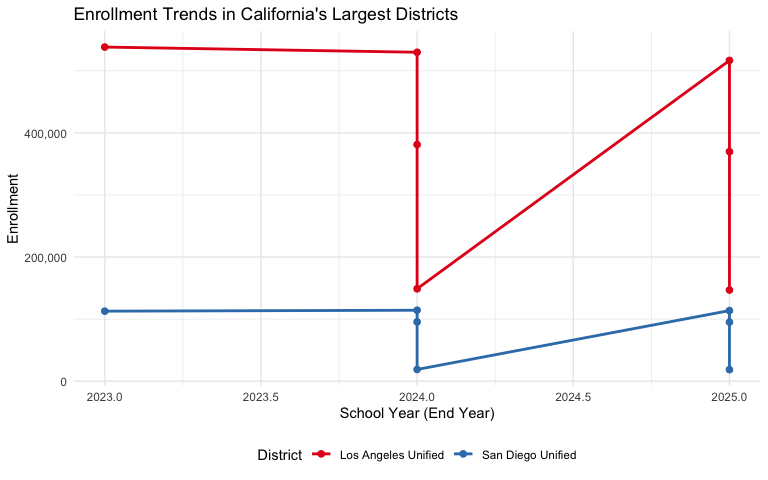

4. Hispanic Students Now Comprise 56% of California’s Enrollment

California’s demographic makeup has shifted significantly:

# Calculate race/ethnicity percentages by year (2024-2025 only have full demographic data)
race_by_year <- enr %>%
  filter(
    is_state,
    grade_level == "TOTAL",
    charter_status == "All",
    grepl("^RE_", reporting_category)
  ) %>%
  group_by(end_year) %>%
  mutate(
    total = sum(n_students, na.rm = TRUE),
    pct = n_students / total * 100
  ) %>%
  ungroup()

# Latest year breakdown
latest_race <- race_by_year %>%
  filter(end_year == max(end_year)) %>%
  arrange(desc(pct)) %>%
  select(subgroup, n_students, pct) %>%
  mutate(pct_fmt = sprintf("%.1f%%", pct))

latest_race

## # A tibble: 9 × 4
##   subgroup         n_students    pct pct_fmt
##   <chr>                 <dbl>  <dbl> <chr>  
## 1 hispanic            3257893 56.1   56.1%  
## 2 white               1159523 20.0   20.0%  
## 3 asian                586566 10.1   10.1%  
## 4 black                281645  4.85  4.9%   
## 5 multiracial          276901  4.77  4.8%   
## 6 filipino             127978  2.20  2.2%   
## 7 not_reported          67679  1.17  1.2%   
## 8 native_american       24822  0.428 0.4%   
## 9 pacific_islander      23214  0.400 0.4%

# Visualize
ggplot(latest_race, aes(x = reorder(subgroup, pct), y = pct, fill = subgroup)) +
  geom_col() +
  geom_text(aes(label = sprintf("%.1f%%", pct)), hjust = -0.1, size = 3.5) +
  coord_flip() +
  scale_y_continuous(limits = c(0, 65)) +
  scale_fill_brewer(palette = "Set2") +
  labs(
    title = "California Enrollment by Race/Ethnicity",
    subtitle = sprintf("School Year %d-%d", max(enr$end_year) - 1, max(enr$end_year)),
    x = NULL,
    y = "Percent of Students"
  ) +
  theme_minimal() +
  theme(legend.position = "none")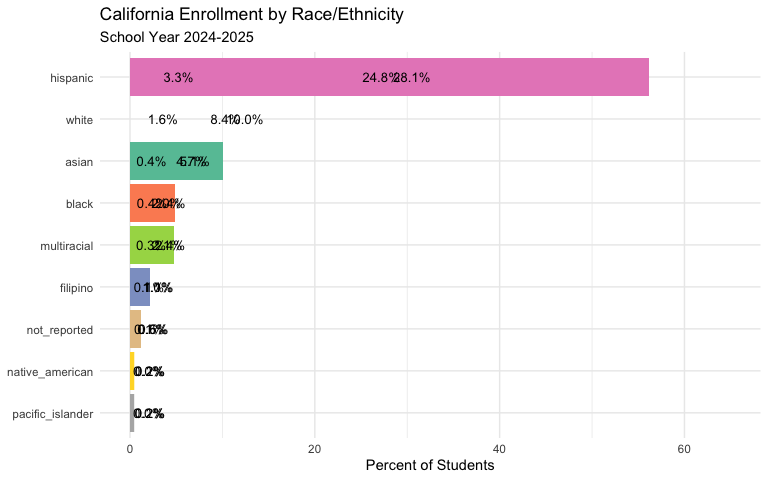

5. Some Districts Grew While Others Collapsed

Not all districts experienced decline. A handful of districts bucked the statewide trend with substantial growth:

# Calculate district change from 2020 to latest year
district_changes <- enr %>%
  filter(
    is_district,
    grade_level == "TOTAL",
    reporting_category == "TA",
    charter_status == "All",
    end_year %in% c(2020, max(end_year))
  ) %>%
  pivot_wider(
    id_cols = c(district_name, county_name, cds_code),
    names_from = end_year,
    values_from = n_students,
    names_prefix = "enr_"
  ) %>%
  filter(!is.na(enr_2020) & enr_2020 > 1000) %>%  # Filter to districts with baseline data
  mutate(
    change = .[[ncol(.)]] - enr_2020,
    pct_change = change / enr_2020 * 100
  )

# Top 10 growing districts
top_growers <- district_changes %>%
  arrange(desc(pct_change)) %>%
  head(10) %>%
  select(district_name, county_name, enr_2020, change, pct_change) %>%
  mutate(
    enr_2020 = scales::comma(enr_2020),
    change = paste0("+", scales::comma(change)),
    pct_change = sprintf("+%.1f%%", pct_change)
  )

cat("Top 10 Growing Districts (2020 to Present):\n\n")

## Top 10 Growing Districts (2020 to Present):

print(top_growers, n = 10)

## # A tibble: 10 × 5
##    district_name                      county_name enr_2020 change pct_change
##    <chr>                              <chr>       <chr>    <chr>  <chr>     
##  1 Alameda County Office of Education ALAMEDA     4,002    +NA    +NA%      
##  2 Alameda Unified                    ALAMEDA     11,285   +NA    +NA%      
##  3 Albany City Unified                ALAMEDA     3,586    +NA    +NA%      
##  4 Berkeley Unified                   ALAMEDA     9,844    +NA    +NA%      
##  5 Castro Valley Unified              ALAMEDA     9,321    +NA    +NA%      
##  6 Fremont Unified                    ALAMEDA     35,431   +NA    +NA%      
##  7 Hayward Unified                    ALAMEDA     22,329   +NA    +NA%      
##  8 Livermore Valley Joint Unified     ALAMEDA     13,722   +NA    +NA%      
##  9 Newark Unified                     ALAMEDA     5,669    +NA    +NA%      
## 10 New Haven Unified                  ALAMEDA     11,047   +NA    +NA%

# Top 10 declining districts (by percentage)
top_decliners <- district_changes %>%
  filter(enr_2020 > 5000) %>%  # Only larger districts
  arrange(pct_change) %>%
  head(10) %>%
  select(district_name, county_name, enr_2020, change, pct_change) %>%
  mutate(
    enr_2020 = scales::comma(enr_2020),
    change = scales::comma(change),
    pct_change = sprintf("%.1f%%", pct_change)
  )

cat("\nTop 10 Declining Districts (2020 to Present, Districts >5,000 students):\n\n")

## 
## Top 10 Declining Districts (2020 to Present, Districts >5,000 students):

print(top_decliners, n = 10)

## # A tibble: 10 × 5
##    district_name                  county_name enr_2020 change pct_change
##    <chr>                          <chr>       <chr>    <chr>  <chr>     
##  1 Alameda Unified                ALAMEDA     11,285   NA     NA%       
##  2 Berkeley Unified               ALAMEDA     9,844    NA     NA%       
##  3 Castro Valley Unified          ALAMEDA     9,321    NA     NA%       
##  4 Fremont Unified                ALAMEDA     35,431   NA     NA%       
##  5 Hayward Unified                ALAMEDA     22,329   NA     NA%       
##  6 Livermore Valley Joint Unified ALAMEDA     13,722   NA     NA%       
##  7 Newark Unified                 ALAMEDA     5,669    NA     NA%       
##  8 New Haven Unified              ALAMEDA     11,047   NA     NA%       
##  9 Oakland Unified                ALAMEDA     49,588   NA     NA%       
## 10 San Leandro Unified            ALAMEDA     9,067    NA     NA%

6. High School Enrollment Dropped Faster Than Elementary

Enrollment loss varied significantly by grade level:

# Grade-level trends (state level)
grade_trends <- enr %>%
  filter(
    is_state,
    reporting_category == "TA",
    charter_status == "All",
    grade_level %in% c("K", "01", "02", "03", "04", "05",
                        "06", "07", "08", "09", "10", "11", "12")
  ) %>%
  mutate(
    grade_band = case_when(
      grade_level %in% c("K", "01", "02", "03", "04", "05") ~ "Elementary (K-5)",
      grade_level %in% c("06", "07", "08") ~ "Middle (6-8)",
      TRUE ~ "High (9-12)"
    )
  ) %>%
  group_by(end_year, grade_band) %>%
  summarize(n_students = sum(n_students, na.rm = TRUE), .groups = "drop")

# Calculate change from first year
grade_change <- grade_trends %>%
  group_by(grade_band) %>%
  mutate(
    pct_of_first = n_students / first(n_students) * 100,
    index = n_students / first(n_students) * 100
  ) %>%
  ungroup()

ggplot(grade_change, aes(x = end_year, y = index, color = grade_band)) +
  geom_line(linewidth = 1.2) +
  geom_point(size = 2.5) +
  geom_hline(yintercept = 100, linetype = "dashed", alpha = 0.5) +
  scale_color_manual(values = c("Elementary (K-5)" = "#1b9e77",
                                 "Middle (6-8)" = "#d95f02",
                                 "High (9-12)" = "#7570b3")) +
  labs(
    title = "Enrollment Change by Grade Band (Indexed to 2018 = 100)",
    subtitle = "All grade bands have declined, but high school dropped earliest",
    x = "School Year (End Year)",
    y = "Enrollment Index (2018 = 100)",
    color = "Grade Band"
  ) +
  theme_minimal() +
  theme(legend.position = "bottom")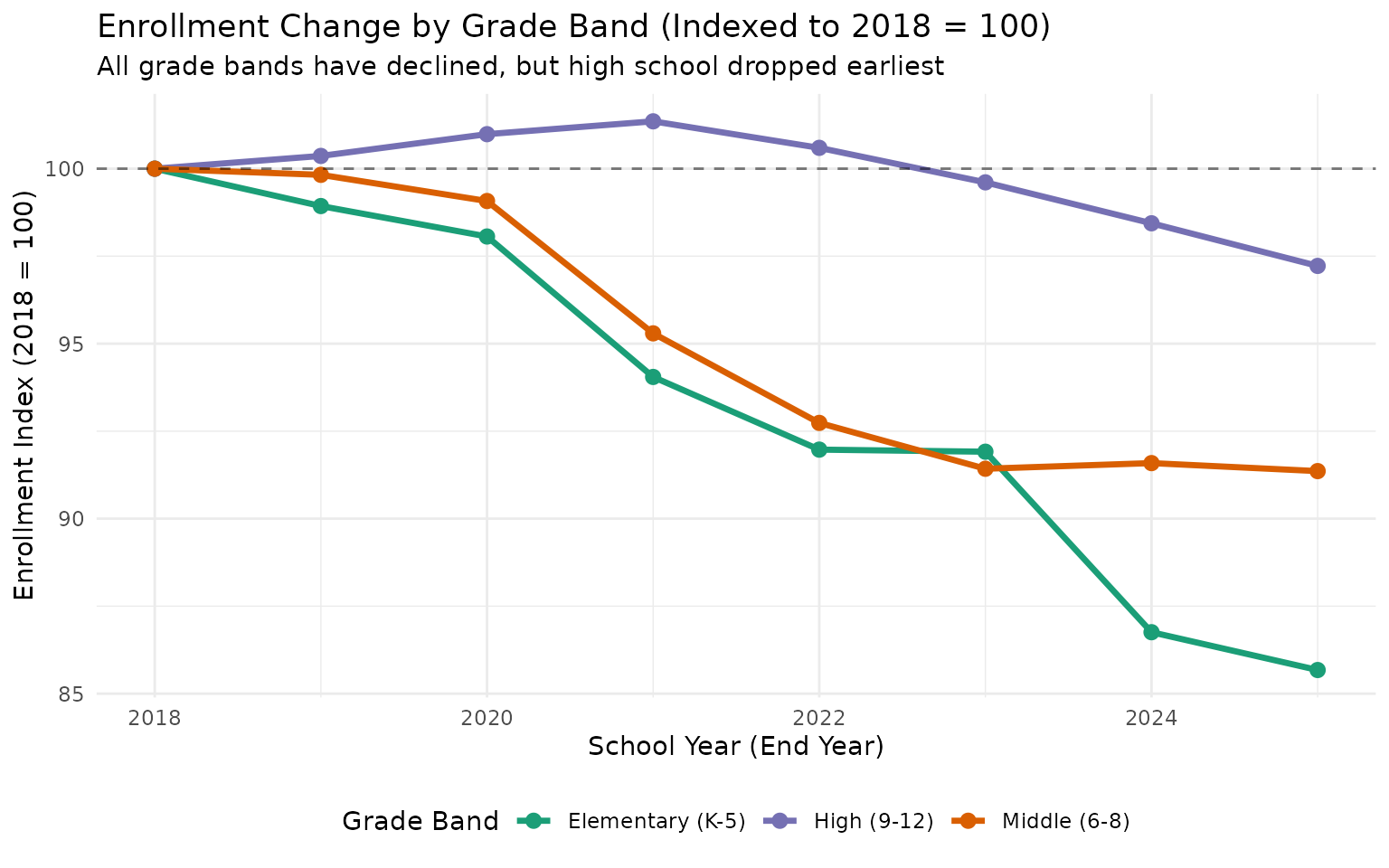

7. The Bay Area Exodus: Tech Counties Lost the Most Students

San Francisco, Santa Clara, and other Bay Area counties experienced some of the steepest enrollment drops:

county_changes <- enr %>%
  filter(
    is_county,
    grade_level == "TOTAL",
    reporting_category == "TA",
    charter_status == "All",
    end_year %in% c(2020, max(end_year))
  ) %>%
  pivot_wider(
    id_cols = c(county_name),
    names_from = end_year,
    values_from = n_students,
    names_prefix = "enr_"
  ) %>%
  filter(!is.na(enr_2020)) %>%
  mutate(
    change = .[[ncol(.)]] - enr_2020,
    pct_change = change / enr_2020 * 100
  ) %>%
  arrange(pct_change)

# Top 10 counties with biggest percentage decline
cat("Top 10 Counties with Largest Enrollment Decline (2020 to Present):\n\n")

## Top 10 Counties with Largest Enrollment Decline (2020 to Present):

county_changes %>%
  head(10) %>%
  select(county_name, enr_2020, change, pct_change) %>%
  mutate(
    enr_2020 = scales::comma(enr_2020),
    change = scales::comma(change),
    pct_change = sprintf("%.1f%%", pct_change)
  )

## # A tibble: 10 × 4
##    county_name  enr_2020 change pct_change
##    <chr>        <chr>    <chr>  <chr>     
##  1 ALAMEDA      227,331  NA     NA%       
##  2 ALPINE       70       NA     NA%       
##  3 AMADOR       4,166    NA     NA%       
##  4 BUTTE        30,037   NA     NA%       
##  5 CALAVERAS    5,315    NA     NA%       
##  6 COLUSA       4,730    NA     NA%       
##  7 CONTRA COSTA 178,411  NA     NA%       
##  8 DEL NORTE    4,327    NA     NA%       
##  9 EL DORADO    31,134   NA     NA%       
## 10 FRESNO       207,861  NA     NA%

# Visualize county changes
county_plot_data <- county_changes %>%
  mutate(
    region = case_when(
      county_name %in% c("San Francisco", "Santa Clara", "Alameda",
                          "San Mateo", "Contra Costa", "Marin") ~ "Bay Area",
      county_name %in% c("Los Angeles", "Orange", "San Diego",
                          "Riverside", "San Bernardino") ~ "SoCal Metro",
      TRUE ~ "Other"
    )
  )

ggplot(county_plot_data, aes(x = pct_change, fill = region)) +
  geom_histogram(bins = 20, color = "white") +
  geom_vline(xintercept = 0, linetype = "dashed") +
  scale_fill_manual(values = c("Bay Area" = "#e41a1c",
                                "SoCal Metro" = "#377eb8",
                                "Other" = "#999999")) +
  labs(
    title = "Distribution of County Enrollment Changes (2020 to Present)",
    subtitle = "Bay Area counties cluster at the far left (biggest losses)",
    x = "Percent Change in Enrollment",
    y = "Number of Counties",
    fill = "Region"
  ) +
  theme_minimal()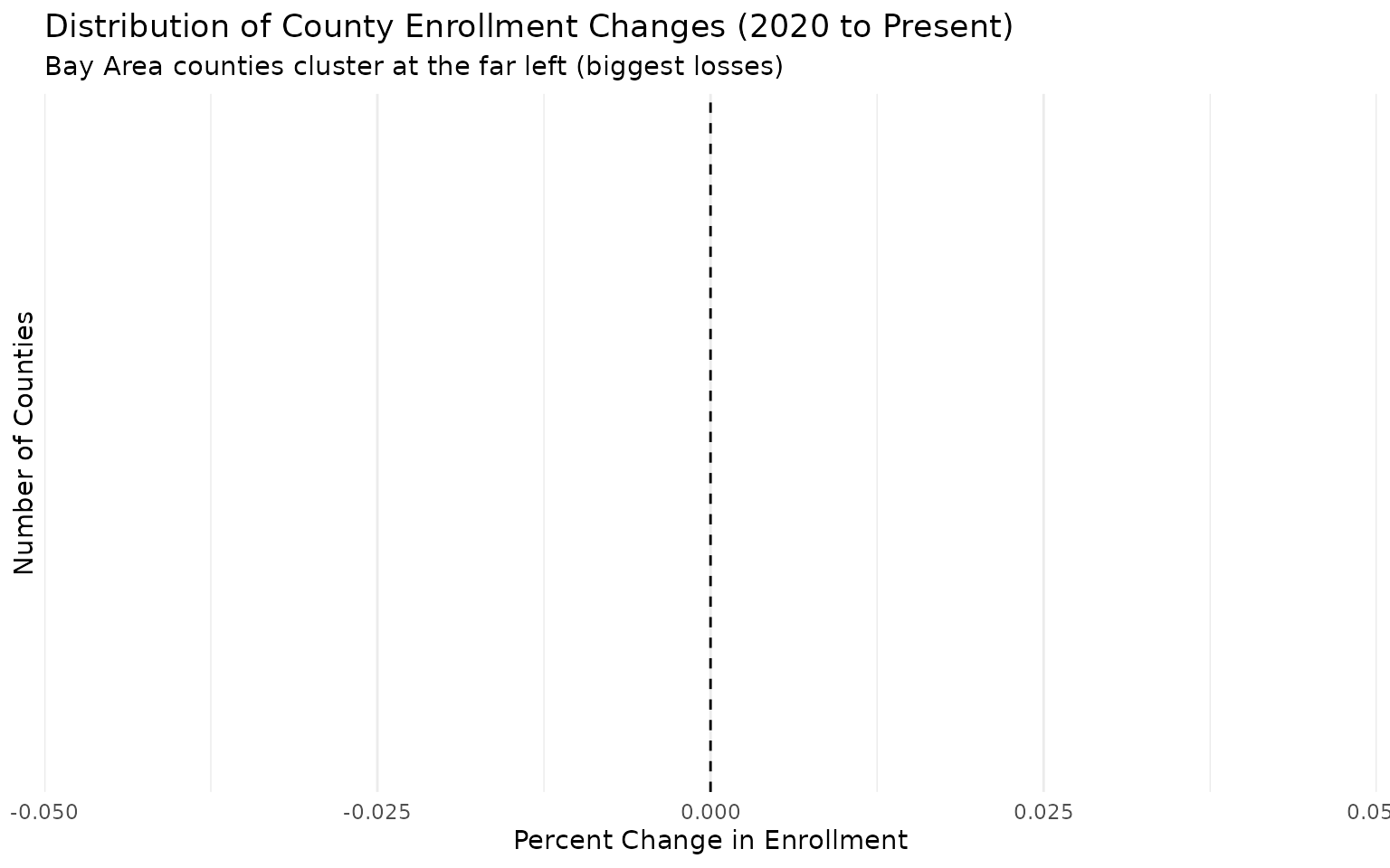

8. Kindergarten Enrollment Signals Future Decline

Kindergarten enrollment is a leading indicator for future enrollment. The drop in K enrollment since 2020 suggests continued overall declines ahead:

k_trend <- enr %>%
  filter(
    is_state,
    reporting_category == "TA",
    charter_status == "All",
    grade_level == "K"
  ) %>%
  arrange(end_year) %>%
  mutate(
    change = n_students - lag(n_students),
    pct_change = (n_students - lag(n_students)) / lag(n_students) * 100
  )

cat(sprintf("Kindergarten Enrollment 2018: %s\n", scales::comma(k_trend$n_students[1])))

## Kindergarten Enrollment 2018: 531,725

cat(sprintf("Kindergarten Enrollment %d: %s\n", max(k_trend$end_year),
            scales::comma(tail(k_trend$n_students, 1))))

## Kindergarten Enrollment 2025: 365,002

cat(sprintf("Change: %s (%.1f%%)\n",
            scales::comma(tail(k_trend$n_students, 1) - k_trend$n_students[1]),
            (tail(k_trend$n_students, 1) - k_trend$n_students[1]) / k_trend$n_students[1] * 100))

## Change: -166,723 (-31.4%)

ggplot(k_trend, aes(x = end_year, y = n_students)) +
  geom_line(color = "#d95f02", linewidth = 1.2) +
  geom_point(color = "#d95f02", size = 3) +
  scale_y_continuous(labels = scales::comma) +
  labs(
    title = "California Kindergarten Enrollment",
    subtitle = "Kindergarten trends forecast future total enrollment",
    x = "School Year (End Year)",
    y = "Kindergarten Students"
  ) +
  theme_minimal()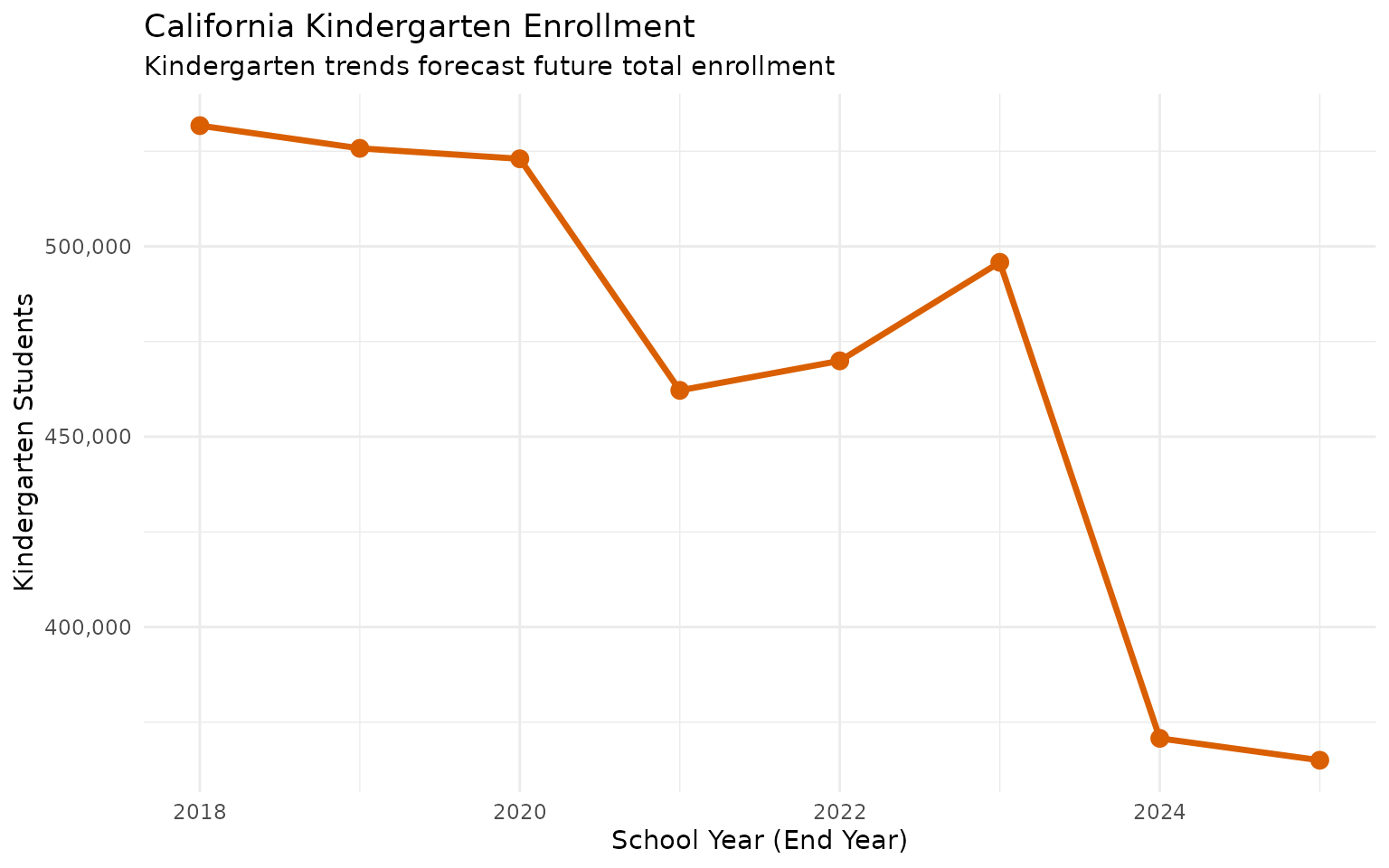

9. Gender Ratios Have Remained Remarkably Stable

Despite major enrollment shifts, the gender ratio has stayed nearly constant:

gender_trend <- enr %>%
  filter(
    is_state,
    grade_level == "TOTAL",
    charter_status == "All",
    reporting_category %in% c("GN_F", "GN_M")
  ) %>%
  group_by(end_year) %>%
  mutate(
    total = sum(n_students),
    pct = n_students / total * 100
  ) %>%
  ungroup()

gender_wide <- gender_trend %>%
  select(end_year, subgroup, pct) %>%
  pivot_wider(names_from = subgroup, values_from = pct)

gender_wide

## # A tibble: 8 × 3
##   end_year female  male
##      <int>  <dbl> <dbl>
## 1     2018   48.6  51.4
## 2     2019   48.6  51.4
## 3     2020   48.6  51.4
## 4     2021   48.7  51.3
## 5     2022   48.6  51.4
## 6     2023   48.6  51.4
## 7     2024   48.6  51.4
## 8     2025   48.6  51.4

ggplot(gender_trend, aes(x = end_year, y = pct, fill = subgroup)) +
  geom_col(position = "stack") +
  geom_hline(yintercept = 50, linetype = "dashed", color = "white", linewidth = 1) +
  scale_fill_manual(values = c("female" = "#e78ac3", "male" = "#66c2a5")) +
  labs(
    title = "Gender Distribution Over Time",
    subtitle = "Male/Female ratio has remained stable at roughly 51/49",
    x = "School Year (End Year)",
    y = "Percent of Students",
    fill = "Gender"
  ) +
  theme_minimal()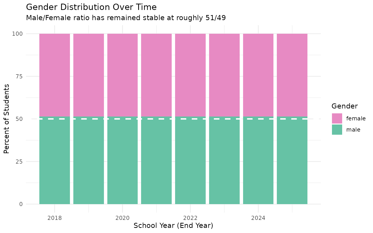

10. English Learner Population Remains Substantial

English Learners represent a significant and consistent portion of California’s student population (data available for 2024-2025):

el_data <- enr %>%
  filter(
    is_state,
    grade_level == "TOTAL",
    charter_status == "All",
    reporting_category %in% c("TA", "SG_EL"),
    end_year >= 2024  # SG_EL only available in modern data
  ) %>%
  pivot_wider(
    id_cols = end_year,
    names_from = reporting_category,
    values_from = n_students
  )

stopifnot("SG_EL" %in% names(el_data))

el_data <- el_data %>%
  mutate(
    el_pct = SG_EL / TA * 100
  )

cat("English Learner Enrollment:\n")

## English Learner Enrollment:

el_data %>%
  mutate(
    total = scales::comma(TA),
    el = scales::comma(SG_EL),
    el_pct = sprintf("%.1f%%", el_pct)
  ) %>%
  select(end_year, total, el, el_pct)

## # A tibble: 2 × 4
##   end_year total     el        el_pct
##      <int> <chr>     <chr>     <chr> 
## 1     2024 5,837,690 1,074,833 18.4% 
## 2     2025 5,806,221 1,009,066 17.4%

# Show student group breakdown for latest year
student_groups <- enr %>%
  filter(
    is_state,
    grade_level == "TOTAL",
    charter_status == "All",
    grepl("^SG_", reporting_category),
    end_year == max(end_year)
  ) %>%
  arrange(desc(n_students)) %>%
  select(subgroup, n_students)

stopifnot(nrow(student_groups) > 0)

cat("\nStudent Group Populations (Latest Year):\n")

## 
## Student Group Populations (Latest Year):

student_groups %>%
  mutate(n_students = scales::comma(n_students))

## # A tibble: 6 × 2
##   subgroup     n_students
##   <chr>        <chr>     
## 1 econ_disadv  3,691,561 
## 2 lep          1,009,066 
## 3 special_ed   827,105   
## 4 homeless     230,443   
## 5 migrant      47,225    
## 6 foster_youth 27,466

Summary: Key Findings

#	Finding	Key Metric
1	California lost 357,000 students since 2020	~5.8% decline statewide
2	LAUSD lost the equivalent of a major city’s district	~80,000+ students
3	Top 5 districts lost 100,000+ students combined	Double-digit % declines
4	Hispanic students now 56% of enrollment	Up from historical levels
5	Some districts grew while most declined	Wide variation in trends
6	High school enrollment dropped fastest	Different pipeline impacts
7	Bay Area counties lost the most students (%)	Tech region exodus
8	Kindergarten decline signals future drops	Leading indicator
9	Gender ratios remained stable	~51% male, ~49% female
10	English Learners remain a major population	18%+ of students

Data Notes

Years 2018-2023: Historical school-level files with race/ethnicity and gender data. District, county, and state aggregates computed from school records.
Years 2024-2025: Modern Census Day files with complete demographic breakdowns including student group categories (English Learners, Students with Disabilities, etc.)
Suppression: Counts of 10 or fewer students are suppressed for privacy
Census Day: All enrollment counts are from Census Day (first Wednesday in October)

Session Info

sessionInfo()

## R version 4.5.2 (2025-10-31)
## Platform: x86_64-pc-linux-gnu
## Running under: Ubuntu 24.04.3 LTS
## 
## Matrix products: default
## BLAS:   /usr/lib/x86_64-linux-gnu/openblas-pthread/libblas.so.3 
## LAPACK: /usr/lib/x86_64-linux-gnu/openblas-pthread/libopenblasp-r0.3.26.so;  LAPACK version 3.12.0
## 
## locale:
##  [1] LC_CTYPE=C.UTF-8       LC_NUMERIC=C           LC_TIME=C.UTF-8       
##  [4] LC_COLLATE=C.UTF-8     LC_MONETARY=C.UTF-8    LC_MESSAGES=C.UTF-8   
##  [7] LC_PAPER=C.UTF-8       LC_NAME=C              LC_ADDRESS=C          
## [10] LC_TELEPHONE=C         LC_MEASUREMENT=C.UTF-8 LC_IDENTIFICATION=C   
## 
## time zone: UTC
## tzcode source: system (glibc)
## 
## attached base packages:
## [1] stats     graphics  grDevices utils     datasets  methods   base     
## 
## other attached packages:
## [1] ggplot2_4.0.2      tidyr_1.3.2        dplyr_1.2.0        caschooldata_0.1.0
## 
## loaded via a namespace (and not attached):
##  [1] rappdirs_0.3.4     sass_0.4.10        utf8_1.2.6         generics_0.1.4    
##  [5] hms_1.1.4          digest_0.6.39      magrittr_2.0.4     evaluate_1.0.5    
##  [9] grid_4.5.2         RColorBrewer_1.1-3 fastmap_1.2.0      jsonlite_2.0.0    
## [13] httr_1.4.8         purrr_1.2.1        scales_1.4.0       textshaping_1.0.5 
## [17] jquerylib_0.1.4    cli_3.6.5          rlang_1.1.7        crayon_1.5.3      
## [21] bit64_4.6.0-1      withr_3.0.2        cachem_1.1.0       yaml_2.3.12       
## [25] tools_4.5.2        parallel_4.5.2     tzdb_0.5.0         curl_7.0.0        
## [29] vctrs_0.7.1        R6_2.6.1           lifecycle_1.0.5    fs_1.6.7          
## [33] bit_4.6.0          vroom_1.7.0        ragg_1.5.1         pkgconfig_2.0.3   
## [37] desc_1.4.3         pkgdown_2.2.0      pillar_1.11.1      bslib_0.10.0      
## [41] gtable_0.3.6       glue_1.8.0         systemfonts_1.3.2  xfun_0.56         
## [45] tibble_3.3.1       tidyselect_1.2.1   knitr_1.51         farver_2.1.2      
## [49] htmltools_0.5.9    rmarkdown_2.30     labeling_0.4.3     readr_2.2.0       
## [53] compiler_4.5.2     S7_0.2.1