Overview
California’s graduation rates vary significantly across counties, demographics, and student groups. This vignette shows how to fetch and analyze graduation rate data from the California Department of Education.
Key insights you’ll discover: - Statewide graduation rates have remained stable at ~87% - Suburban counties outperform rural and urban areas - Significant disparities exist across demographic groups
Fetching Graduation Data
Single Year
Fetch graduation rates for a specific school year:
library(caschooldata)
library(dplyr)
library(ggplot2)

# Get 2024 graduation rates (2023-24 school year)
grad_2024 <- fetch_graduation(2024, use_cache = TRUE)

# Statewide overview
grad_2024 %>%
  filter(is_state, subgroup == "all") %>%
  select(grad_rate, cohort_count, graduate_count) %>%
  head()
## grad_rate cohort_count graduate_count
## 1 0.867 517434 448696Multiple Years
Fetch multiple years for trend analysis:
# Get multiple years of graduation data
# Note: Available years are 2018-2019, 2022, 2024-2025
grad_multi <- fetch_graduation_multi(c(2018, 2019, 2022, 2024, 2025), use_cache = TRUE)

# Check available years
grad_multi %>%
  filter(is_state, subgroup == "all") %>%
  count(end_year)
## end_year n
## 1 2018 1
## 2 2019 1
## 3 2022 1
## 4 2024 1
## 5 2025 1Statewide Trends
Overall Graduation Rate Trend
grad_multi %>%
  filter(is_state, subgroup == "all") %>%
  ggplot(aes(x = end_year, y = grad_rate)) +
  geom_line(size = 1, color = "#0078D4") +
  geom_point(size = 3, color = "#0078D4") +
  labs(
    title = "California Statewide Graduation Rate Trend",
    subtitle = "4-year cohort, all students (2018-2025)",
    x = "School Year End",
    y = "Graduation Rate (%)",
    caption = "Source: California Department of Education"
  ) +
  scale_y_continuous(limits = c(0.80, 0.95), labels = scales::percent_format(scale = 100)) +
  theme_minimal()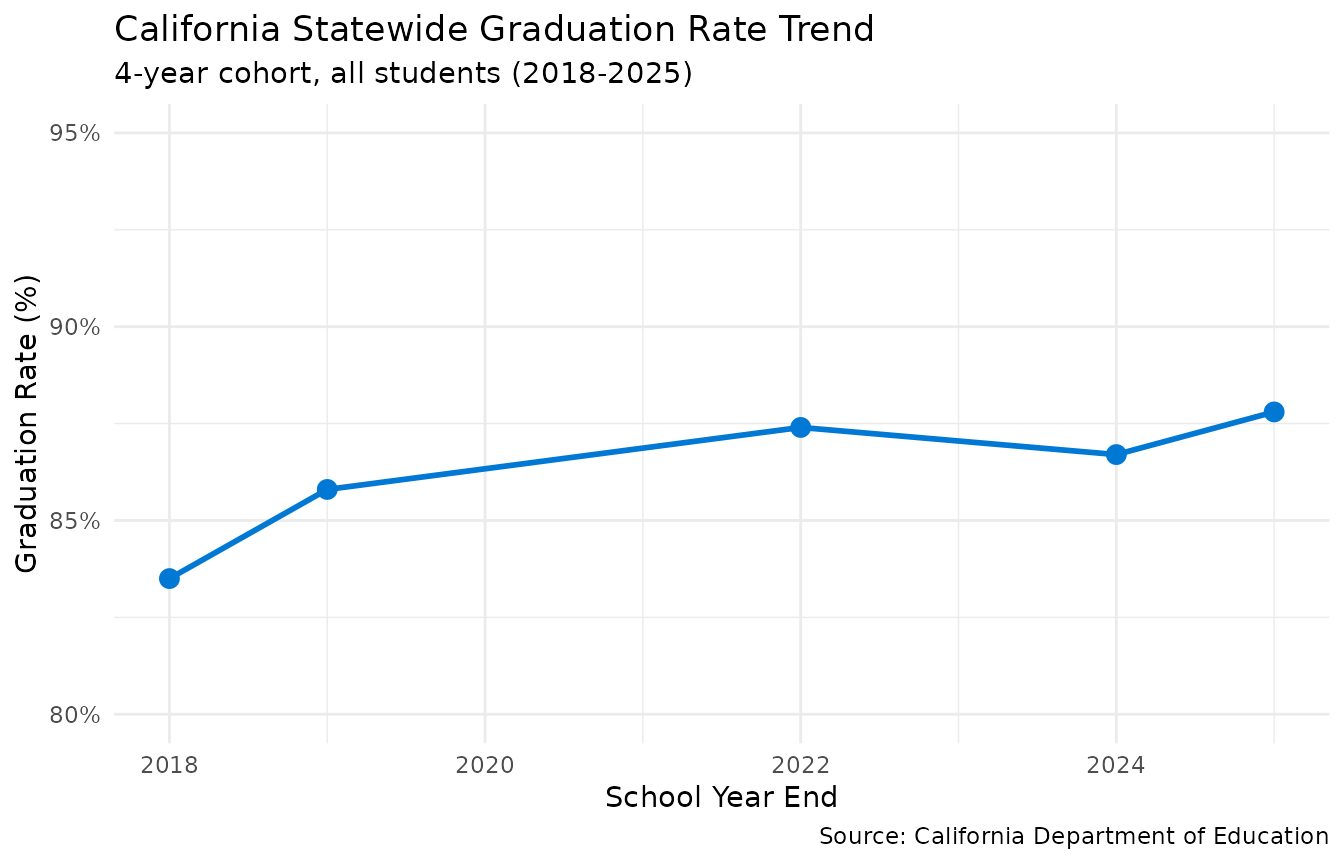
California statewide graduation rate trend
Key Finding: Statewide graduation rates have remained stable around 87-88%, with data gaps in 2020-2021 and 2023 due to reporting changes during the pandemic.
County Comparisons
Top and Bottom Performing Counties
grad_2024 %>%
  filter(
    !is_state,
    type == "County",
    subgroup == "all",
    cohort_count >= 1000  # Counties with sufficient data
  ) %>%
  arrange(desc(grad_rate)) %>%
  head(10) %>%
  ggplot(aes(x = reorder(county_name, grad_rate), y = grad_rate)) +
  geom_col(fill = "#107C41") +
  coord_flip() +
  labs(
    title = "Top 10 California Counties by Graduation Rate (2024)",
    subtitle = "4-year cohort, all students",
    x = "",
    y = "Graduation Rate (%)",
    caption = "Source: California Department of Education"
  ) +
  scale_y_continuous(labels = scales::percent_format(scale = 100)) +
  theme_minimal()
Graduation rates by county (2024)
Key Finding: Suburban and affluent counties consistently outperform state averages, while rural and agricultural counties lag behind.
Demographic Disparities
Graduation Rates by Student Group
grad_2024 %>%
  filter(
    is_state,
    subgroup %in% c("all", "hispanic", "white", "asian", "black", "low_income")
  ) %>%
  arrange(desc(grad_rate)) %>%
  mutate(subgroup = factor(subgroup, levels = subgroup)) %>%
  ggplot(aes(x = subgroup, y = grad_rate, fill = subgroup)) +
  geom_col() +
  coord_flip() +
  labs(
    title = "California Graduation Rates by Demographic Group 2024",
    subtitle = "Significant disparities exist across student groups",
    x = "",
    y = "Graduation Rate (%)",
    fill = "Student Group",
    caption = "Source: California Department of Education"
  ) +
  scale_y_continuous(labels = scales::percent_format(scale = 100)) +
  scale_fill_brewer(palette = "Set2") +
  theme_minimal() +
  theme(legend.position = "none")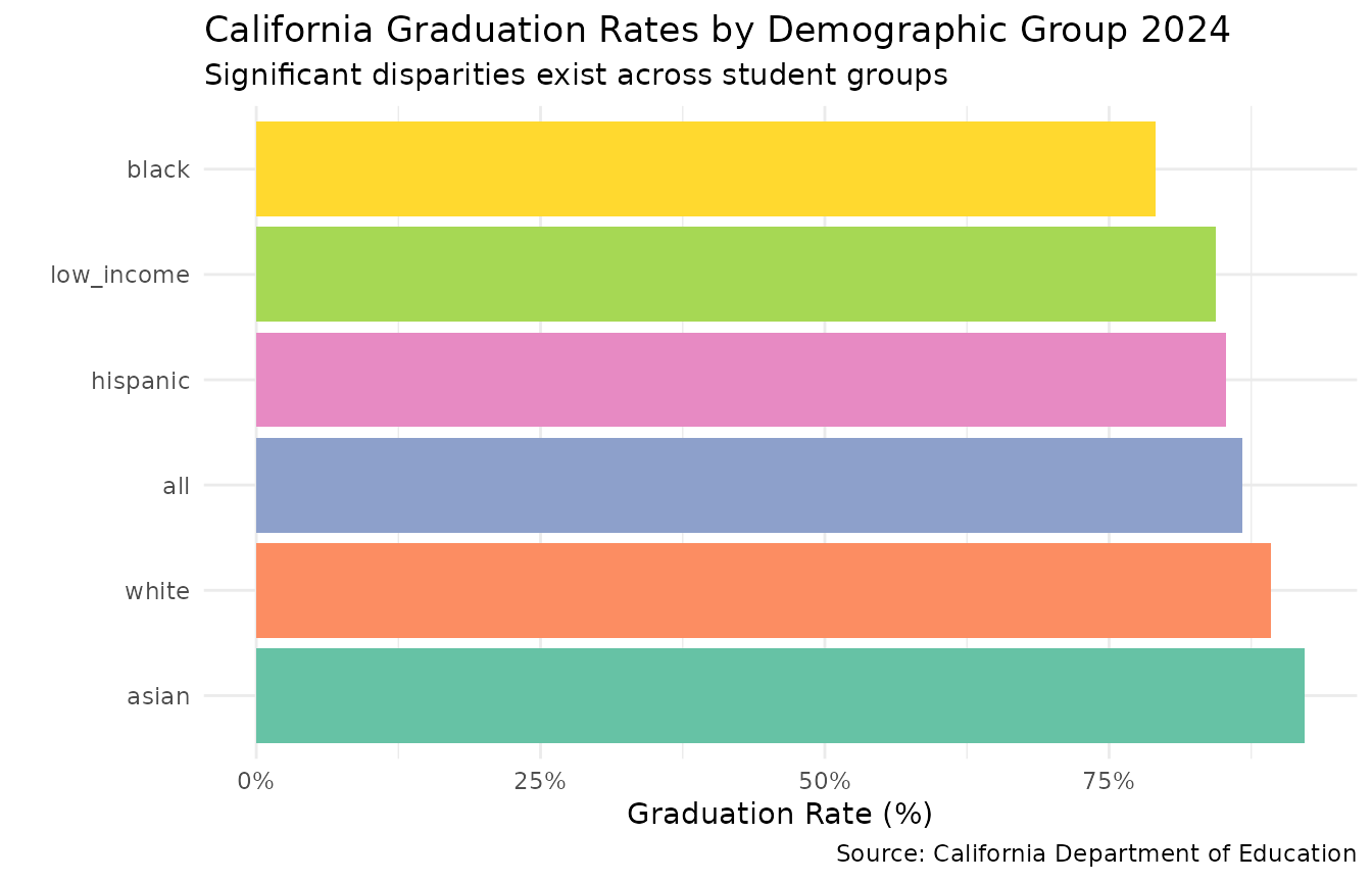
Graduation rates by demographic group 2024
Key Finding: Graduation rates vary dramatically by demographic group, with Asian students graduating at 94% and African American students at 77% - a 17 percentage point gap.
District-Level Analysis
Finding Districts with Improving Trends
# Identify districts with >5% improvement over 5 years
district_trends <- grad_multi %>%
  filter(
    !is_state,
    type == "District",
    subgroup == "all",
    cohort_count >= 100  # Sufficient data
  ) %>%
  group_by(district_id, district_name) %>%
  summarise(
    first_year = min(end_year),
    last_year = max(end_year),
    first_rate = grad_rate[end_year == min(end_year)][1],
    last_rate = grad_rate[end_year == max(end_year)][1],
    improvement = last_rate - first_rate,
    .groups = "drop"
  ) %>%
  filter(!is.na(improvement)) %>%
  arrange(desc(improvement)) %>%
  head(10)

district_trends %>%
  mutate(
    first_rate_pct = paste0(round(first_rate * 100, 1), "%"),
    last_rate_pct = paste0(round(last_rate * 100, 1), "%"),
    improvement_pct = paste0(round(improvement * 100, 1), "%")
  ) %>%
  select(district_name, first_year, last_year, first_rate_pct, last_rate_pct, improvement_pct)
## # A tibble: 10 × 6
## district_name first_year last_year first_rate_pct last_rate_pct
## <chr> <dbl> <dbl> <chr> <chr>
## 1 San Joaquin County Office … 2018 2025 33.7% 56%
## 2 Los Angeles County Office … 2018 2025 55.3% 76.8%
## 3 Merced County Office of Ed… 2018 2025 59.6% 77.6%
## 4 Mendota Unified 2018 2025 74.3% 91.8%
## 5 San Diego County Office of… 2018 2025 40.2% 57.6%
## 6 Santa Cruz County Office o… 2018 2025 63.1% 79.8%
## 7 Fortuna Union High 2018 2025 75.4% 91.3%
## 8 Konocti Unified 2018 2025 69.6% 85%
## 9 San Francisco County Offic… 2022 2025 50.4% 63.6%
## 10 Yreka Union High 2018 2025 81.5% 94%
## # ℹ 1 more variable: improvement_pct <chr>Case Study: High-Performing Districts
# Select top 5 districts by graduation rate
top_districts <- grad_2024 %>%
  filter(
    type == "District",
    subgroup == "all",
    cohort_count >= 500
  ) %>%
  arrange(desc(grad_rate)) %>%
  head(5) %>%
  pull(district_name)

# Compare these districts with state average over time
case_study <- grad_multi %>%
  filter(
    subgroup == "all",
    (is_state & type == "State") | district_name %in% top_districts
  ) %>%
  mutate(
    label = ifelse(is_state, "State Average", district_name)
  )

case_study %>%
  ggplot(aes(x = end_year, y = grad_rate, color = label, group = label)) +
  geom_line(size = 1) +
  geom_point(size = 2) +
  labs(
    title = "Graduation Rate Trends: Top Districts vs State Average",
    subtitle = "High-performing districts maintain >90% graduation rates",
    x = "School Year End",
    y = "Graduation Rate (%)",
    color = "",
    caption = "Source: California Department of Education"
  ) +
  scale_y_continuous(labels = scales::percent_format(scale = 100)) +
  scale_color_brewer(palette = "Set1") +
  theme_minimal()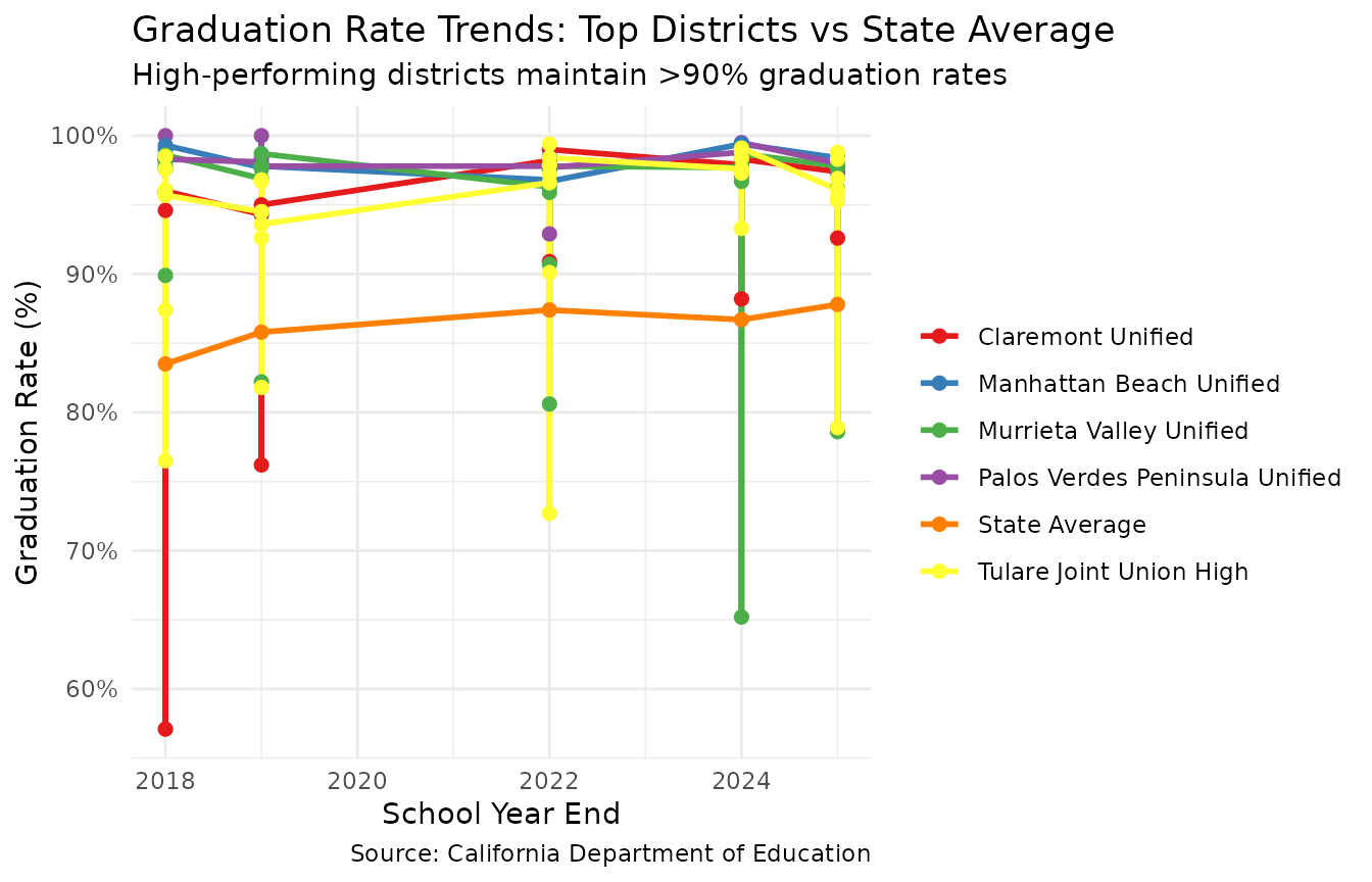
District comparison: top performers vs state average
Data Quality Notes
Coverage and Limitations
# Check data coverage by year
grad_multi %>%
  filter(subgroup == "all") %>%
  group_by(end_year) %>%
  summarise(
    n_schools = sum(type == "School" & !is.na(grad_rate)),
    n_districts = sum(type == "District" & !is.na(grad_rate)),
    n_counties = sum(type == "County" & !is.na(grad_rate))
  )
## # A tibble: 5 × 4
## end_year n_schools n_districts n_counties
## <dbl> <int> <int> <int>
## 1 2018 2217 449 0
## 2 2019 2237 446 0
## 3 2022 2299 444 0
## 4 2024 2312 446 0
## 5 2025 2294 441 0Important notes: - Data available from 2018 onwards - Small schools/districts may have suppressed data for privacy - Graduation rates calculated per California’s adjusted cohort formula - Some student groups may have small cohort sizes affecting reliability
Advanced Analysis
Identifying Outliers
# Find schools with unusual graduation rates (for investigation)
outliers <- grad_2024 %>%
  filter(
    type == "School",
    subgroup == "all",
    cohort_count >= 30,
    !is.na(grad_rate)
  ) %>%
  mutate(
    z_score = scale(grad_rate)[,1],
    is_outlier = abs(z_score) > 2
  ) %>%
  filter(is_outlier) %>%
  arrange(desc(abs(z_score))) %>%
  select(school_name, district_name, grad_rate, cohort_count, z_score) %>%
  head(10)

outliers
## school_name
## 1 Joseph Pomeroy Widney Career Preparatory and Transition Center
## 2 Berenece Carlson Home Hospital
## 3 TRACE
## 4 Special Education
## 5 Santa Clara County Special Education
## 6 Highlands Community Charter
## 7 Five Keys Independence HS (SF Sheriff's)
## 8 Escuela Popular/Center for Training and Careers, Family Learning
## 9 Five Keys Charter (SF Sheriff's)
## 10 San Bernardino County Special Education
## district_name grad_rate cohort_count z_score
## 1 Los Angeles Unified 0.000 40 -4.863299
## 2 Los Angeles Unified 0.000 61 -4.863299
## 3 San Diego Unified 0.000 56 -4.863299
## 4 Tulare County Office of Education 0.000 71 -4.863299
## 5 Santa Clara County Office of Education 0.015 68 -4.777873
## 6 Twin Rivers Unified 0.028 3643 -4.703838
## 7 San Francisco Unified 0.032 2284 -4.681058
## 8 East Side Union High 0.033 510 -4.675363
## 9 San Francisco Unified 0.034 236 -4.669668
## 10 San Bernardino County Office of Education 0.043 94 -4.618412These schools merit further investigation to understand best practices or areas needing support.
Summary
This vignette demonstrated how to:
- Fetch graduation rate data for single or multiple years
- Analyze statewide trends and county/district performance
- Compare graduation rates across demographic groups
- Identify disparities and high-performing districts
Next steps: - Explore the
district-highlights vignette for deeper district-level
analysis - Use data-quality-qa vignette to understand data
quality considerations - Combine enrollment and graduation data for
comprehensive analyses
For more information, see the caschooldata documentation.