Fetch and analyze California school enrollment, assessment, and graduation data from the California Department of Education in R or Python. 44 years of enrollment data (1982-2025), CAASPP assessment results (2015-2024), and graduation rates (2018-2025) for 5.8 million students across 1,000+ districts.
Part of the njschooldata family.
Full documentation — all 15 stories with interactive charts, getting-started guide, and complete function reference.
Highlights
library(caschooldata)
library(dplyr)
library(tidyr)
library(ggplot2)

# Fetch enrollment data (2018-2025)
years <- 2018:2025
enr <- fetch_enr_multi(years)

# Fetch 2024 assessment data
assess_2024 <- fetch_assess(2024, tidy = TRUE, use_cache = TRUE)
1. California Lost 357,000 Students Since 2020
California public schools have lost over 357,000 students since the pandemic began. This represents a decline of 5.8% in just five years — a city-sized school system gone from the rolls.
state_trend <- enr %>%
  filter(is_state, grade_level == "TOTAL", reporting_category == "TA",
         charter_status == "All") %>%
  arrange(end_year) %>%
  mutate(
    cumulative_change = n_students - first(n_students),
    pct_change = (n_students - first(n_students)) / first(n_students) * 100
  )

# Calculate the specific decline from 2020 peak
peak_2020 <- state_trend %>% filter(end_year == 2020) %>% pull(n_students)
current <- state_trend %>% filter(end_year == max(end_year)) %>% pull(n_students)
decline <- peak_2020 - current

cat(sprintf("Peak enrollment (2020): %s students\n", scales::comma(peak_2020)))
cat(sprintf("Current enrollment: %s students\n", scales::comma(current)))
cat(sprintf("Total decline: %s students (%.1f%%)\n",
            scales::comma(decline),
            decline / peak_2020 * 100))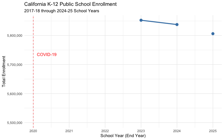
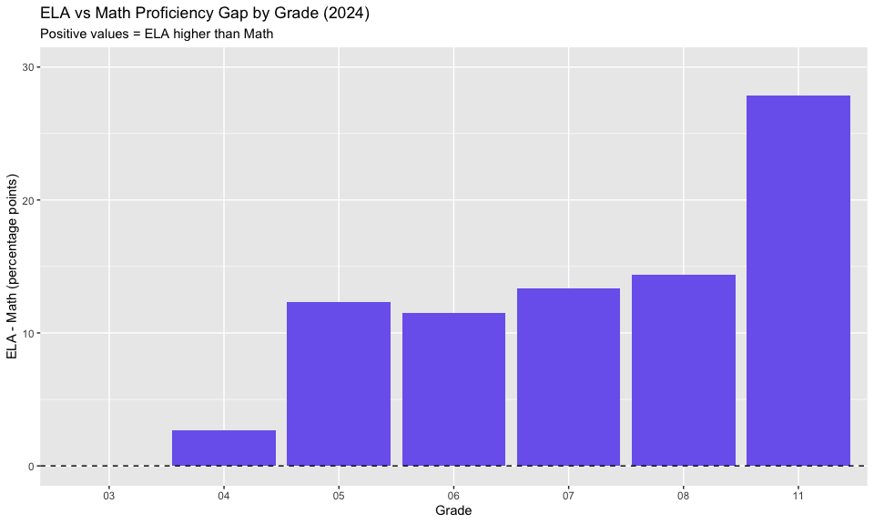
2. 11th graders lead all grades in ELA — but math tells the opposite story
ELA proficiency jumps from 43-47% in grades 3-8 to 55.7% for 11th graders. Math goes the other direction: Grade 3 tops out at 45.6% and falls to just 27.9% by Grade 11.
# ELA proficiency by grade
ela_by_grade <- assess_2024 %>%
  filter(is_state, subject == "ELA",
         metric_type == "pct_met_and_above",
         grade %in% sprintf("%02d", c(3:8, 11))) %>%
  select(grade, metric_value) %>%
  arrange(grade)

ela_by_grade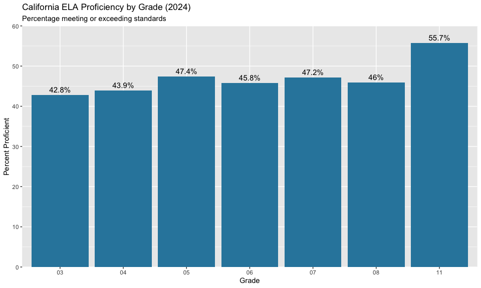
3. The Bay Area Exodus: Tech Counties Lost the Most Students
San Francisco, Santa Clara, and other Bay Area counties experienced some of the steepest enrollment drops:
county_changes <- enr %>%
  filter(
    is_county,
    grade_level == "TOTAL",
    reporting_category == "TA",
    charter_status == "All",
    end_year %in% c(2020, max(end_year))
  ) %>%
  pivot_wider(
    id_cols = c(county_name),
    names_from = end_year,
    values_from = n_students,
    names_prefix = "enr_"
  ) %>%
  filter(!is.na(enr_2020)) %>%
  mutate(
    change = .[[ncol(.)]] - enr_2020,
    pct_change = change / enr_2020 * 100
  ) %>%
  arrange(pct_change)

# Top 10 counties with biggest percentage decline
cat("Top 10 Counties with Largest Enrollment Decline (2020 to Present):\n\n")
county_changes %>%
  head(10) %>%
  select(county_name, enr_2020, change, pct_change) %>%
  mutate(
    enr_2020 = scales::comma(enr_2020),
    change = scales::comma(change),
    pct_change = sprintf("%.1f%%", pct_change)
  )
Data Taxonomy
| Category | Years | Function | Details |
|---|---|---|---|
| Enrollment | 1982-2025 |
fetch_enr() / fetch_enr_multi()
|
State, county, district, school. Race, gender, EL, FRPL, SpEd |
| Assessments | 2015-2024 |
fetch_assess() / fetch_assess_multi()
|
CAASPP ELA & Math. Grades 3-8, 11. State, district, school |
| Graduation | 2018-2025 |
fetch_graduation() / fetch_graduation_multi()
|
State, county, district, school. Race, gender, EL, SpEd, low-income |
| Directory | Current | fetch_directory() |
State, county, district, school. Superintendent, principal, address, phone |
| Per-Pupil Spending | — | — | Not yet available |
| Accountability | — | — | Not yet available |
| Chronic Absence | — | — | Not yet available |
| EL Progress | — | — | Not yet available |
| Special Ed | — | — | Not yet available |
See DATA-CATEGORY-TAXONOMY.md for what each category covers.
Quick Start
R
# install.packages("remotes")
remotes::install_github("almartin82/caschooldata")

library(caschooldata)
library(dplyr)

# Fetch one year
enr_2025 <- fetch_enr(2025)

# Fetch recent years (2018-2025)
enr_recent <- fetch_enr_multi(2018:2025)

# Fetch ALL 44 years of data (1982-2025)
enr_all <- fetch_enr_multi(1982:2025)

# State totals
enr_2025 %>%
  filter(is_state, subgroup == "total_enrollment", grade_level == "TOTAL")

# District breakdown
enr_2025 %>%
  filter(is_district, subgroup == "total_enrollment", grade_level == "TOTAL") %>%
  arrange(desc(n_students))

# Demographics by district
enr_2025 %>%
  filter(is_district, grade_level == "TOTAL", grepl("^RE_", reporting_category)) %>%
  group_by(district_name, subgroup) %>%
  summarize(n = sum(n_students))
Python
import pycaschooldata as ca

# Check available years
years = ca.get_available_years()
print(f"Data available from {years['min_year']} to {years['max_year']}")

# Fetch one year
enr_2025 = ca.fetch_enr(2025)

# Fetch multiple years
enr_recent = ca.fetch_enr_multi([2023, 2024, 2025])

# State totals
state_total = enr_2025[
    (enr_2025['is_state'] == True) &
    (enr_2025['grade_level'] == 'TOTAL') &
    (enr_2025['subgroup'] == 'total_enrollment')
]

# District breakdown
district_totals = enr_2025[
    (enr_2025['is_district'] == True) &
    (enr_2025['grade_level'] == 'TOTAL') &
    (enr_2025['subgroup'] == 'total_enrollment')
].sort_values('n_students', ascending=False)
Explore More
- Full documentation
- Enrollment trends — 10 stories
- Assessment analysis — 15 stories
- Graduation rates
- Function reference
Data Notes
Enrollment Data
- Source: California Department of Education DataQuest and Data Files
- Census Day: All enrollment counts are from Census Day (first Wednesday in October)
- Suppression: Counts of 10 or fewer students are suppressed for privacy
- Charter Status: Modern files (2024+) report charter and non-charter separately; historical files aggregate all schools
Assessment Data (CAASPP)
- Source: CAASPP Research Files Portal
- Years Available: 2015-2019, 2021-2024 (no 2020 due to COVID-19)
- Grades Tested: 3-8 and 11 for ELA and Mathematics
- Suppression: Groups with fewer than 11 students are not reported
- Performance Levels: Standard Exceeded, Standard Met, Standard Nearly Met, Standard Not Met
Deeper Dive
4. LAUSD Has Lost the Equivalent of a Major City’s School District
Los Angeles Unified, the nation’s second-largest school district, has experienced dramatic enrollment losses:
lausd <- enr %>%
  filter(
    is_district,
    grade_level == "TOTAL",
    reporting_category == "TA",
    charter_status == "All",
    grepl("Los Angeles Unified", district_name, ignore.case = TRUE)
  ) %>%
  arrange(end_year) %>%
  mutate(
    change = n_students - lag(n_students),
    cumulative_change = n_students - first(n_students)
  )

cat(sprintf("LAUSD 2018: %s students\n", scales::comma(lausd$n_students[1])))
cat(sprintf("LAUSD 2025: %s students\n", scales::comma(tail(lausd$n_students, 1))))
cat(sprintf("Total loss: %s students (%.1f%%)\n",
            scales::comma(abs(tail(lausd$cumulative_change, 1))),
            abs(tail(lausd$cumulative_change, 1)) / lausd$n_students[1] * 100))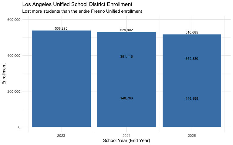
5. The Top 5 Districts Lost Over 100,000 Students Combined
California’s five largest districts all face significant enrollment challenges:
# Find the 5 largest districts (by 2025 enrollment)
top5_districts <- enr %>%
  filter(
    is_district,
    end_year == max(end_year),
    grade_level == "TOTAL",
    reporting_category == "TA",
    charter_status == "All"
  ) %>%
  arrange(desc(n_students)) %>%
  head(5) %>%
  pull(district_name)

top5_trend <- enr %>%
  filter(
    is_district,
    grade_level == "TOTAL",
    reporting_category == "TA",
    charter_status == "All",
    district_name %in% top5_districts
  ) %>%
  arrange(district_name, end_year)

# Calculate change from first to last year
top5_change <- top5_trend %>%
  group_by(district_name) %>%
  summarize(
    enr_first = first(n_students),
    enr_last = last(n_students),
    change = last(n_students) - first(n_students),
    pct_change = (last(n_students) - first(n_students)) / first(n_students) * 100,
    .groups = "drop"
  ) %>%
  arrange(change)

top5_change %>%
  mutate(
    district_name = gsub(" School District$| Unified$| Unified School District$", "", district_name),
    change_fmt = scales::comma(change),
    pct_fmt = sprintf("%.1f%%", pct_change)
  ) %>%
  select(district_name, enr_first, enr_last, change_fmt, pct_fmt)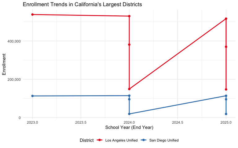
6. Hispanic Students Now Comprise 56% of California’s Enrollment
California’s demographic makeup has shifted significantly:
# Calculate race/ethnicity percentages by year (2024-2025 only have full demographic data)
race_by_year <- enr %>%
  filter(
    is_state,
    grade_level == "TOTAL",
    charter_status == "All",
    grepl("^RE_", reporting_category)
  ) %>%
  group_by(end_year) %>%
  mutate(
    total = sum(n_students, na.rm = TRUE),
    pct = n_students / total * 100
  ) %>%
  ungroup()

# Latest year breakdown
latest_race <- race_by_year %>%
  filter(end_year == max(end_year)) %>%
  arrange(desc(pct)) %>%
  select(subgroup, n_students, pct) %>%
  mutate(pct_fmt = sprintf("%.1f%%", pct))

latest_race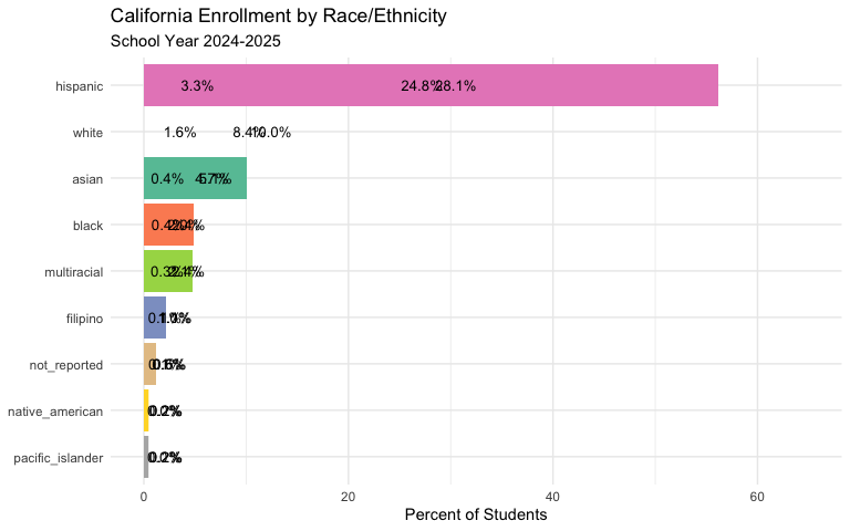
7. Some Districts Grew While Others Collapsed
Not all districts experienced decline. A handful of districts bucked the statewide trend with substantial growth:
# Calculate district change from 2020 to latest year
district_changes <- enr %>%
  filter(
    is_district,
    grade_level == "TOTAL",
    reporting_category == "TA",
    charter_status == "All",
    end_year %in% c(2020, max(end_year))
  ) %>%
  pivot_wider(
    id_cols = c(district_name, county_name, cds_code),
    names_from = end_year,
    values_from = n_students,
    names_prefix = "enr_"
  ) %>%
  filter(!is.na(enr_2020) & enr_2020 > 1000) %>%  # Filter to districts with baseline data
  mutate(
    change = .[[ncol(.)]] - enr_2020,
    pct_change = change / enr_2020 * 100
  )

# Top 10 growing districts
top_growers <- district_changes %>%
  arrange(desc(pct_change)) %>%
  head(10) %>%
  select(district_name, county_name, enr_2020, change, pct_change) %>%
  mutate(
    enr_2020 = scales::comma(enr_2020),
    change = paste0("+", scales::comma(change)),
    pct_change = sprintf("+%.1f%%", pct_change)
  )

cat("Top 10 Growing Districts (2020 to Present):\n\n")
print(top_growers, n = 10)

# Top 10 declining districts (by percentage)
top_decliners <- district_changes %>%
  filter(enr_2020 > 5000) %>%  # Only larger districts
  arrange(pct_change) %>%
  head(10) %>%
  select(district_name, county_name, enr_2020, change, pct_change) %>%
  mutate(
    enr_2020 = scales::comma(enr_2020),
    change = scales::comma(change),
    pct_change = sprintf("%.1f%%", pct_change)
  )

cat("\nTop 10 Declining Districts (2020 to Present, Districts >5,000 students):\n\n")
print(top_decliners, n = 10)
8. High School Enrollment Dropped Faster Than Elementary
Enrollment loss varied significantly by grade level:
# Grade-level trends (state level)
grade_trends <- enr %>%
  filter(
    is_state,
    reporting_category == "TA",
    charter_status == "All",
    grade_level %in% c("K", "01", "02", "03", "04", "05",
                        "06", "07", "08", "09", "10", "11", "12")
  ) %>%
  mutate(
    grade_band = case_when(
      grade_level %in% c("K", "01", "02", "03", "04", "05") ~ "Elementary (K-5)",
      grade_level %in% c("06", "07", "08") ~ "Middle (6-8)",
      TRUE ~ "High (9-12)"
    )
  ) %>%
  group_by(end_year, grade_band) %>%
  summarize(n_students = sum(n_students, na.rm = TRUE), .groups = "drop")

# Calculate change from first year
grade_change <- grade_trends %>%
  group_by(grade_band) %>%
  mutate(
    pct_of_first = n_students / first(n_students) * 100,
    index = n_students / first(n_students) * 100
  ) %>%
  ungroup()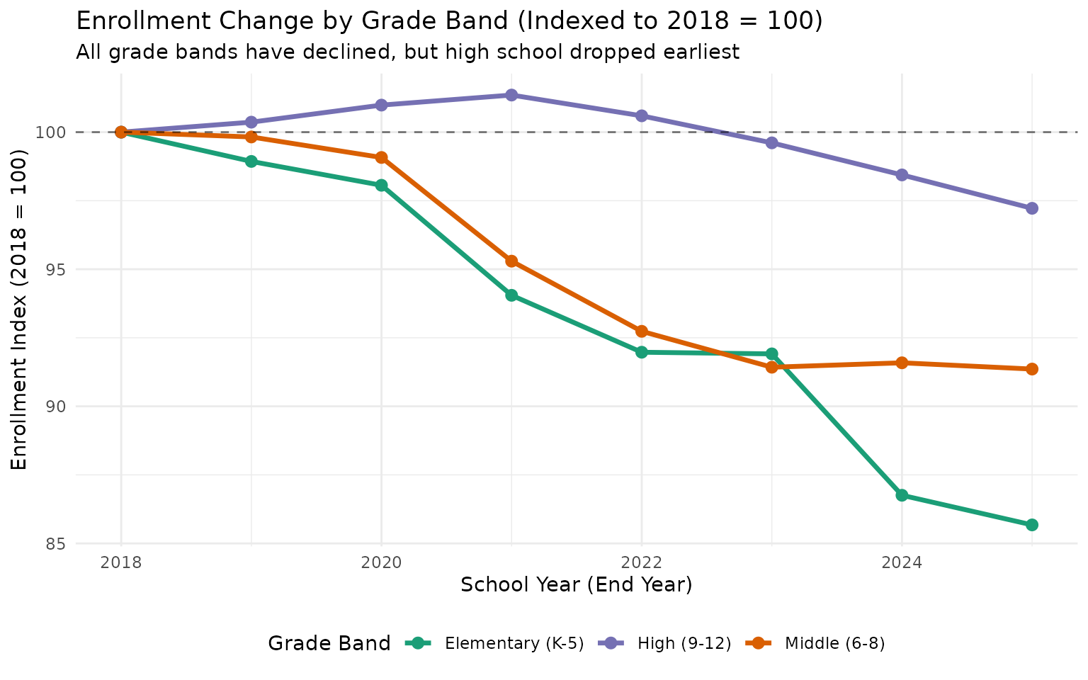
9. Kindergarten Enrollment Signals Future Decline
Kindergarten enrollment is a leading indicator for future enrollment. The drop in K enrollment since 2020 suggests continued overall declines ahead:
k_trend <- enr %>%
  filter(
    is_state,
    reporting_category == "TA",
    charter_status == "All",
    grade_level == "K"
  ) %>%
  arrange(end_year) %>%
  mutate(
    change = n_students - lag(n_students),
    pct_change = (n_students - lag(n_students)) / lag(n_students) * 100
  )

cat(sprintf("Kindergarten Enrollment 2018: %s\n", scales::comma(k_trend$n_students[1])))
cat(sprintf("Kindergarten Enrollment %d: %s\n", max(k_trend$end_year),
            scales::comma(tail(k_trend$n_students, 1))))
cat(sprintf("Change: %s (%.1f%%)\n",
            scales::comma(tail(k_trend$n_students, 1) - k_trend$n_students[1]),
            (tail(k_trend$n_students, 1) - k_trend$n_students[1]) / k_trend$n_students[1] * 100))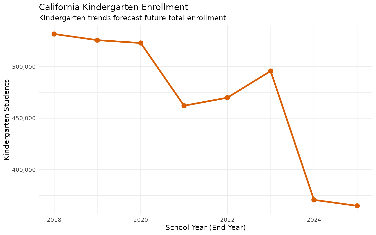
10. Gender Ratios Have Remained Remarkably Stable
Despite major enrollment shifts, the gender ratio has stayed nearly constant:
gender_trend <- enr %>%
  filter(
    is_state,
    grade_level == "TOTAL",
    charter_status == "All",
    reporting_category %in% c("GN_F", "GN_M")
  ) %>%
  group_by(end_year) %>%
  mutate(
    total = sum(n_students),
    pct = n_students / total * 100
  ) %>%
  ungroup()

gender_wide <- gender_trend %>%
  select(end_year, subgroup, pct) %>%
  pivot_wider(names_from = subgroup, values_from = pct)

gender_wide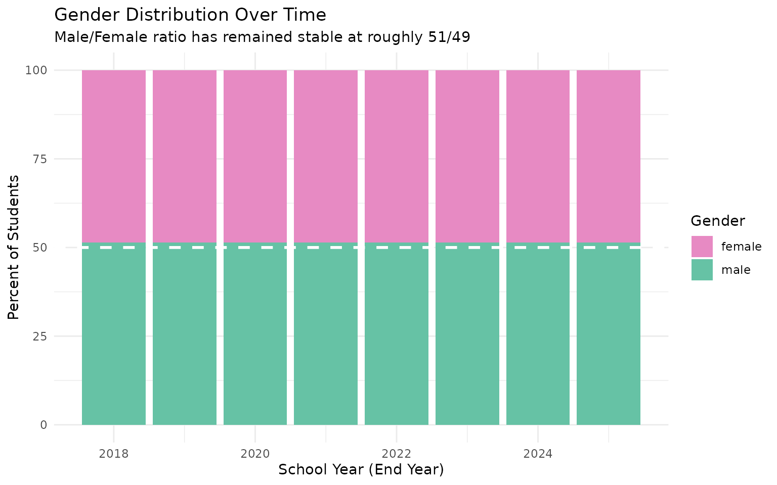
11. English Learner Population Remains Substantial
English Learners represent a significant and consistent portion of California’s student population (data available for 2024-2025):
el_data <- enr %>%
  filter(
    is_state,
    grade_level == "TOTAL",
    charter_status == "All",
    reporting_category %in% c("TA", "SG_EL"),
    end_year >= 2024  # SG_EL only available in modern data
  ) %>%
  pivot_wider(
    id_cols = end_year,
    names_from = reporting_category,
    values_from = n_students
  )

stopifnot("SG_EL" %in% names(el_data))

el_data <- el_data %>%
  mutate(
    el_pct = SG_EL / TA * 100
  )

cat("English Learner Enrollment:\n")
el_data %>%
  mutate(
    total = scales::comma(TA),
    el = scales::comma(SG_EL),
    el_pct = sprintf("%.1f%%", el_pct)
  ) %>%
  select(end_year, total, el, el_pct)

# Show student group breakdown for latest year
student_groups <- enr %>%
  filter(
    is_state,
    grade_level == "TOTAL",
    charter_status == "All",
    grepl("^SG_", reporting_category),
    end_year == max(end_year)
  ) %>%
  arrange(desc(n_students)) %>%
  select(subgroup, n_students)

stopifnot(nrow(student_groups) > 0)

cat("\nStudent Group Populations (Latest Year):\n")
student_groups %>%
  mutate(n_students = scales::comma(n_students))
12. Statewide proficiency: 47% in ELA, 36% in Math
Across all tested grades, California students showed a persistent 11-point gap between ELA and Math proficiency in 2024.
# State-level proficiency by subject (all grades combined, grade == "13" in CAASPP)
state_all_grades <- assess_2024 %>%
  filter(is_state, grade == "13", metric_type == "pct_met_and_above") %>%
  select(subject, metric_value)

state_all_grades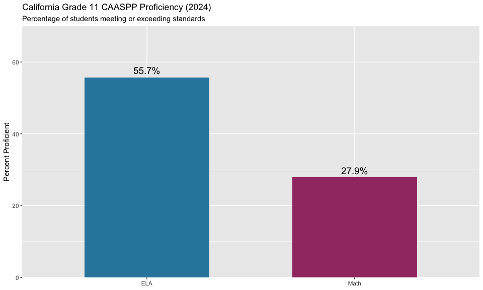
13. Math proficiency drops dramatically by middle school
Math proficiency peaks in Grade 3-4 at around 45% and falls to under 32% by Grade 8.
# Math proficiency by grade
math_by_grade <- assess_2024 %>%
  filter(is_state, subject == "Math",
         metric_type == "pct_met_and_above",
         grade %in% sprintf("%02d", c(3:8, 11))) %>%
  select(grade, metric_value) %>%
  arrange(grade)

math_by_grade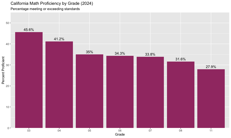
14. Multi-year trends: Recovery from COVID
Proficiency rates are recovering from the 2021 pandemic lows but remain below 2019 levels.
# Fetch multiple years
assess_multi <- fetch_assess_multi(c(2019, 2021, 2022, 2023, 2024),
                                    tidy = TRUE, use_cache = TRUE)

# State-level trend
state_trend <- assess_multi %>%
  filter(is_state, grade == "11", metric_type == "pct_met_and_above") %>%
  select(end_year, subject, metric_value) %>%
  arrange(subject, end_year)

state_trend %>%
  pivot_wider(names_from = subject, values_from = metric_value)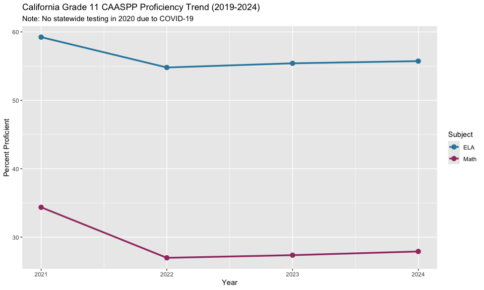
15. ELA-Math gap is consistent across grades
The ELA advantage over Math proficiency is remarkably consistent (10-20 points) across all tested grades.
# ELA-Math gap by grade
ela_math_gap <- assess_2024 %>%
  filter(is_state, metric_type == "pct_met_and_above",
         grade %in% sprintf("%02d", c(3:8, 11))) %>%
  select(grade, subject, metric_value) %>%
  pivot_wider(names_from = subject, values_from = metric_value) %>%
  mutate(gap = ELA - Math)

ela_math_gap