Exploring New Hampshire Statewide Assessment Results
Source:vignettes/newhampshire-assessment.Rmd
newhampshire-assessment.RmdNew Hampshire’s statewide assessment results reach back to 2009. The data spans two very different testing regimes: the New England Common Assessment Program (NECAP, 2009-2014) and the Smarter Balanced / NH SAS assessments (2015-2025). 2020 is absent statewide because the federal COVID assessment waiver cancelled spring testing.
A few things to keep in mind throughout:
-
NH DOE never publishes a raw student count. Every
count is reported as a 5-wide band (e.g.
"35 - 40"), son_testedis alwaysNAand the bounds live inn_tested_lower/n_tested_upper. We never invent a point value. -
Suppressed cells are
NA, never 0. A school with fewer than 11 tested students is masked, and that mask is preserved. -
NECAP and Smarter Balanced are not comparable.
Different tests, scales, and cut scores. The
assessment_eracolumn flags the 2014/2015 boundary, and Story 3 below shows exactly why you must not read across it.
# Bundled NH DOE assessment files: 2009-2019 and 2021-2025 (no 2020).
asmt <- fetch_assessment_multi(c(2009:2019, 2021:2025), use_cache = TRUE)
asmt |>
  count(assessment_era, type) |>
  arrange(assessment_era, type)
#>   assessment_era     type      n
#> 1          NECAP   School  27631
#> 2     SBAC_NHSAS District 218964
#> 3     SBAC_NHSAS   School 342716
#> 4     SBAC_NHSAS    State   2281
1. New Hampshire math never recovered from COVID
State-level results are published from 2018 onward (NECAP and the early Smarter Balanced years are reported at the school level only). Across that window, math tells a stark story: statewide proficiency sat at 48% in 2018 and 2019, collapsed to 38% in the 2021 return-to-testing year, and five years later is still stuck at 42%. Reading dipped too, but has nearly clawed its way back.
state_trend <- asmt |>
  filter(
    is_state, grade == "TOTAL", subgroup == "total_enrollment",
    subject %in% c("math", "reading")
  ) |>
  select(end_year, subject, pct_proficient) |>
  arrange(subject, end_year)

stopifnot(nrow(state_trend) > 0)
state_trend
#>    end_year subject pct_proficient
#> 1      2018    math             48
#> 2      2019    math             48
#> 3      2021    math             38
#> 4      2022    math             40
#> 5      2023    math             42
#> 6      2024    math             41
#> 7      2025    math             42
#> 8      2018 reading             58
#> 9      2019 reading             56
#> 10     2021 reading             52
#> 11     2022 reading             51
#> 12     2023 reading             52
#> 13     2024 reading             53
#> 14     2025 reading             55
ggplot(state_trend, aes(end_year, pct_proficient, color = subject)) +
  geom_line(linewidth = 1.1) +
  geom_point(size = 2) +
  geom_vline(xintercept = 2020, linetype = "dotted", color = "grey50") +
  annotate("text", x = 2020, y = 36, label = "2020: no test\n(COVID waiver)",
           size = 3, color = "grey40", hjust = -0.05) +
  scale_color_manual(values = c(math = "#c0392b", reading = "#2c7fb8")) +
  scale_y_continuous(limits = c(30, 65)) +
  labs(
    title = "NH statewide proficiency, all students (SBAC / NH SAS era)",
    subtitle = "Math fell to 38% in 2021 and has not recovered; reading nearly has",
    x = "School year (end)", y = "% proficient (levels 3 & 4)", color = "Subject"
  ) +
  theme_minimal()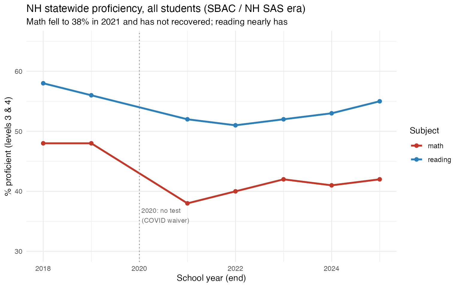
2. A 20-point economic divide in math, baked in before COVID
Economically disadvantaged students (the econ_disadv
subgroup) trail the statewide average by roughly 20 percentage points in
math, every single year. The gap was 21 points in 2018 and was still 19
points in 2025. COVID lowered both lines without meaningfully closing
the distance between them.
ses_gap <- asmt |>
  filter(
    is_state, grade == "TOTAL", subject == "math",
    subgroup %in% c("total_enrollment", "econ_disadv")
  ) |>
  select(end_year, subgroup, pct_proficient) |>
  pivot_wider(names_from = subgroup, values_from = pct_proficient) |>
  mutate(gap = total_enrollment - econ_disadv) |>
  arrange(end_year)

stopifnot(nrow(ses_gap) > 0)
ses_gap
#> # A tibble: 7 × 4
#>   end_year total_enrollment econ_disadv   gap
#>      <int>            <dbl>       <dbl> <dbl>
#> 1     2018               48          27    21
#> 2     2019               48          27    21
#> 3     2021               38          18    20
#> 4     2022               40          21    19
#> 5     2023               42          22    20
#> 6     2024               41          22    19
#> 7     2025               42          23    19
ses_long <- ses_gap |>
  select(end_year, total_enrollment, econ_disadv) |>
  pivot_longer(-end_year, names_to = "group", values_to = "pct")

ggplot(ses_long, aes(end_year, pct, color = group)) +
  geom_line(linewidth = 1.1) +
  geom_point(size = 2) +
  scale_color_manual(
    values = c(total_enrollment = "#2c3e50", econ_disadv = "#e67e22"),
    labels = c(total_enrollment = "All students", econ_disadv = "Econ. disadvantaged")
  ) +
  scale_y_continuous(limits = c(0, 55)) +
  labs(
    title = "NH math proficiency: all students vs. economically disadvantaged",
    subtitle = "A persistent ~20-point gap that COVID did not close",
    x = "School year (end)", y = "% proficient (levels 3 & 4)", color = NULL
  ) +
  theme_minimal()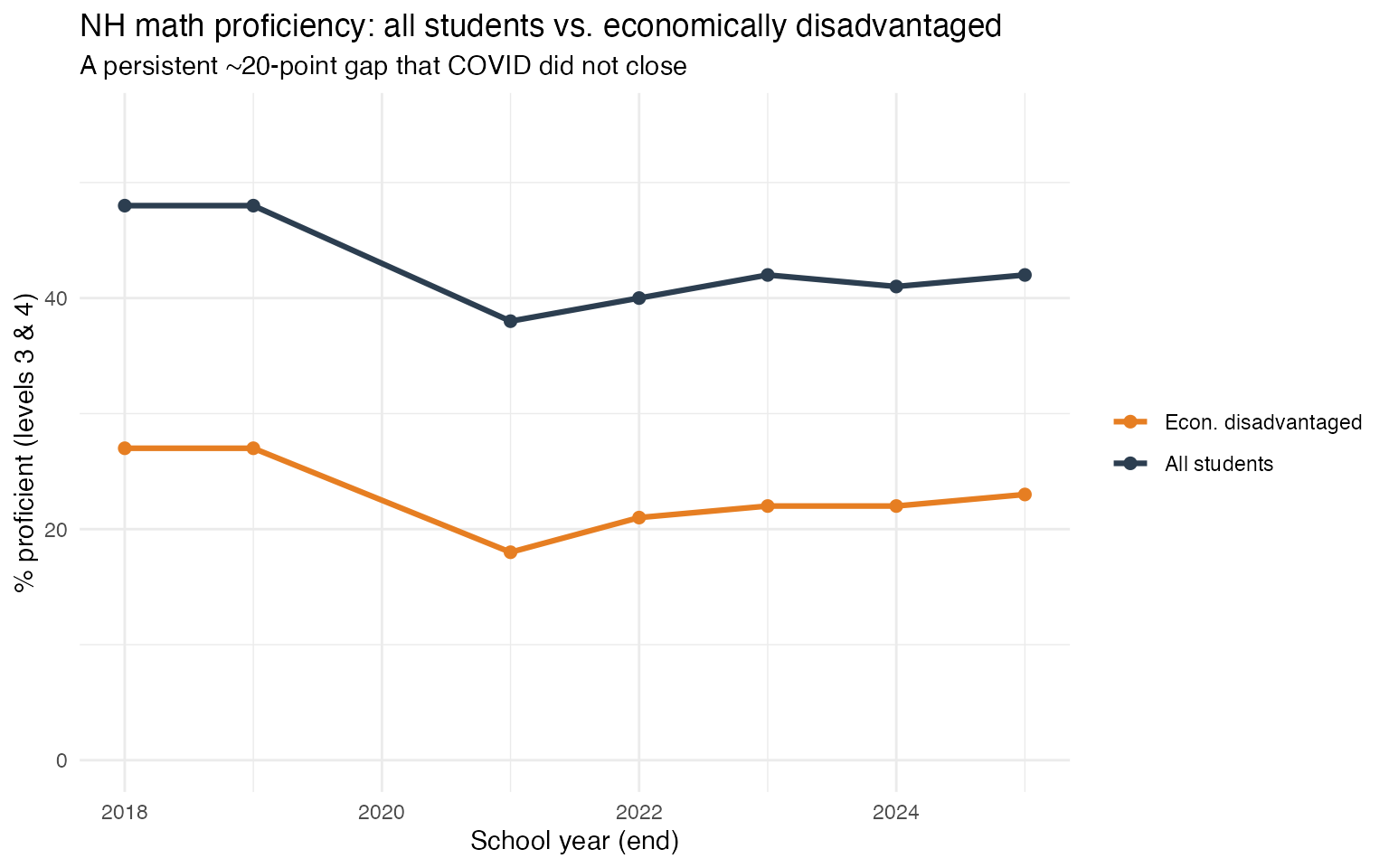
3. The 2015 “cliff” is a test change, not a collapse in learning
In 2015 New Hampshire retired NECAP and adopted the Smarter Balanced
assessment, which uses a substantially higher proficiency bar. Looking
at the median school’s grade-3 math proficiency, the rate appears to
fall off a cliff, from about 71-75% under NECAP (2012-2014) to roughly
53-58% under Smarter Balanced (2015 onward). This drop is an
artifact of the cut-score change, not real learning loss. It is
exactly the kind of comparison the assessment_era flag
exists to prevent. (The later 2021 dip, by contrast, sits entirely
inside the Smarter Balanced era and is comparable, which is why
it reads as a real COVID effect.)
median_g3_math <- asmt |>
  filter(
    type == "School", subject == "math", grade == "03",
    subgroup == "total_enrollment", !is.na(pct_proficient)
  ) |>
  group_by(end_year, assessment_era) |>
  summarise(median_prof = median(pct_proficient), n_schools = n(), .groups = "drop") |>
  arrange(end_year)

stopifnot(nrow(median_g3_math) > 0)
median_g3_math
#> # A tibble: 16 × 4
#>    end_year assessment_era median_prof n_schools
#>       <int> <chr>                <dbl>     <int>
#>  1     2009 NECAP                 72         218
#>  2     2010 NECAP                 75         200
#>  3     2011 NECAP                 77         209
#>  4     2012 NECAP                 74         200
#>  5     2013 NECAP                 75         211
#>  6     2014 NECAP                 71         220
#>  7     2015 SBAC_NHSAS            53         235
#>  8     2016 SBAC_NHSAS            58         232
#>  9     2017 SBAC_NHSAS            55         229
#> 10     2018 SBAC_NHSAS            57.5       234
#> 11     2019 SBAC_NHSAS            59         228
#> 12     2021 SBAC_NHSAS            45         215
#> 13     2022 SBAC_NHSAS            53         229
#> 14     2023 SBAC_NHSAS            53         223
#> 15     2024 SBAC_NHSAS            52         224
#> 16     2025 SBAC_NHSAS            54         225
ggplot(median_g3_math, aes(end_year, median_prof, color = assessment_era)) +
  geom_line(aes(group = 1), linewidth = 0.6, color = "grey70") +
  geom_point(size = 3) +
  geom_vline(xintercept = 2014.5, linetype = "dashed", color = "grey40") +
  annotate("text", x = 2014.5, y = 40, label = "NECAP -> Smarter Balanced\n(not comparable)",
           size = 3, color = "grey30", hjust = 1.02) +
  scale_color_manual(values = c(NECAP = "#16a085", SBAC_NHSAS = "#8e44ad")) +
  labs(
    title = "Median school-level grade-3 math proficiency, by year",
    subtitle = "The 2015 drop reflects a harder test, not falling achievement",
    x = "School year (end)", y = "Median school % proficient", color = "Test regime"
  ) +
  theme_minimal()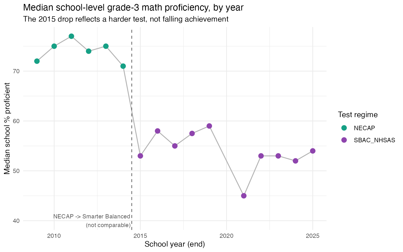
Working with the data
The tidy schema is long: one row per entity x subject x grade x
subgroup. Entity flags (is_state, is_district,
is_school) make filtering simple, and every percentage
column is on a 0-100 scale.
asmt |>
  filter(is_school, subject == "reading", grade == "TOTAL",
         subgroup == "total_enrollment", end_year == 2025) |>
  select(district_name, school_name, n_tested_lower, n_tested_upper,
         pct_proficient, pct_participate, avg_score) |>
  arrange(desc(pct_proficient)) |>
  head(10)
#>                   district_name                  school_name n_tested_lower
#> 1                    Portsmouth          New Franklin School            115
#> 2  Hollis-Brookline Cooperative Hollis-Brookline High School            140
#> 3                       Bedford          Bedford High School            285
#> 4                      Grantham      Grantham Village School            145
#> 5                       Jackson       Jackson Grammar School             20
#> 6                          Lyme       Lyme Elementary School            125
#> 7             Oyster River Coop     Oyster River High School            175
#> 8                       Dresden   Frances C. Richmond School            345
#> 9            Lafayette Regional    Lafayette Regional School             55
#> 10                        Mason      Mason Elementary School             50
#>    n_tested_upper pct_proficient pct_participate avg_score
#> 1             120             88              98        NA
#> 2             145             87              88        NA
#> 3             290             86              90        NA
#> 4             150             86              98        NA
#> 5              25             86             100        NA
#> 6             130             86              98        NA
#> 7             180             86              93        NA
#> 8             350             85              96        NA
#> 9              60             84              98        NA
#> 10             55             84              98        NA
Available subgroups grow over time. The NECAP era (2009-2014) reports all students only; the Smarter Balanced / NH SAS era adds race/ethnicity, gender, economic status, special education, English learners, and additional special populations.
asmt |>
  filter(end_year == 2025) |>
  distinct(subgroup) |>
  arrange(subgroup)
#>                  subgroup
#> 1  asian_pacific_islander
#> 2                   black
#> 3             econ_disadv
#> 4                  female
#> 5             foster_care
#> 6                hispanic
#> 7                homeless
#> 8                     lep
#> 9                    male
#> 10        military_family
#> 11            multiracial
#> 12        native_american
#> 13        not_econ_disadv
#> 14         not_special_ed
#> 15             special_ed
#> 16       total_enrollment
#> 17                  white
sessionInfo()
#> R version 4.5.0 (2025-04-11)
#> Platform: aarch64-apple-darwin22.6.0
#> Running under: macOS 26.1
#>
#> Matrix products: default
#> BLAS:   /opt/homebrew/Cellar/openblas/0.3.30/lib/libopenblasp-r0.3.30.dylib
#> LAPACK: /opt/homebrew/Cellar/r/4.5.0/lib/R/lib/libRlapack.dylib;  LAPACK version 3.12.1
#>
#> locale:
#> [1] en_US.UTF-8/en_US.UTF-8/en_US.UTF-8/C/en_US.UTF-8/en_US.UTF-8
#>
#> time zone: America/New_York
#> tzcode source: internal
#>
#> attached base packages:
#> [1] stats     graphics  grDevices utils     datasets  methods   base
#>
#> other attached packages:
#> [1] testthat_3.3.1     tidyr_1.3.2        ggplot2_4.0.1      dplyr_1.2.1
#> [5] nhschooldata_0.3.4
#>
#> loaded via a namespace (and not attached):
#>  [1] gtable_0.3.6       jsonlite_2.0.0     compiler_4.5.0     brio_1.1.5
#>  [5] tidyselect_1.2.1   jquerylib_0.1.4    systemfonts_1.3.1  scales_1.4.0
#>  [9] textshaping_1.0.4  yaml_2.3.12        fastmap_1.2.0      R6_2.6.1
#> [13] labeling_0.4.3     generics_0.1.4     knitr_1.51         htmlwidgets_1.6.4
#> [17] tibble_3.3.1       desc_1.4.3         bslib_0.9.0        pillar_1.11.1
#> [21] RColorBrewer_1.1-3 rlang_1.3.0        utf8_1.2.6         cachem_1.1.0
#> [25] xfun_0.55          S7_0.2.1           fs_2.1.0           sass_0.4.10
#> [29] otel_0.2.0         cli_3.6.6          withr_3.0.3        pkgdown_2.2.0
#> [33] magrittr_2.0.5     digest_0.6.39      grid_4.5.0         rappdirs_0.3.4
#> [37] lifecycle_1.0.5    vctrs_0.7.3        evaluate_1.0.5     glue_1.8.1
#> [41] farver_2.1.2       codetools_0.2-20   ragg_1.5.0         purrr_1.2.2
#> [45] rmarkdown_2.30     tools_4.5.0        pkgconfig_2.0.3    htmltools_0.5.9